library(geoR)
If the installation directory for the package is the default location for R packages, type:
library(geoR, lib.loc="PATH_TO_geoR")
where "PATH_TO_geoR" is the path to the directory where geoR was installed. If the package is loaded correctly the following message will be displayed:
------------------------------------------------
geoR: functions for geostatistical data analysis
geoR version 1.3-17 is now loaded
------------------------------------------------
Typically, data are stored as an object (a list) of the class "geodata".
An object of this class contains at least the coordinates of data locations and the data values.
Click for information on how to read data from an ASCII (text) file.
We refer to the documentation for the functions as.geodata and read.geodata for more information on how to import/convert data and on the definitions for the class "geodata".
For the examples included in this document we use the data set s100 included in the geoR distribution.
To load this data type:
data(s100)
- A quick summary for the geodata object A quick summary of the data can be obtained typing
- Plotting data locations and values The function plot.geodata shows a 2 x 2 display with data locations (top plots) and data versus coordinates (bottom plots). For an object of the class "geodata" the plot is produced by the command:
- Empirical variograms
summary(s100)which will return a summary of the coordinates and data values like this
$coords.summary
           [,1]       [,2]
min 0.005638006 0.01091027
max 0.983920544 0.99124979

$data.summary
   Min. 1st Qu.  Median    Mean 3rd Qu.    Max.
-1.1680  0.2730  1.1050  0.9307  1.6100  2.8680
Elements covariate, borders and or units.m will be also summarized if present in the geodata object.
plot(s100)
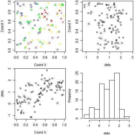
Notice that the top-right plot is produced using the package scatterplot3d. If this package is not installed a histogram of the data will replace this plot.
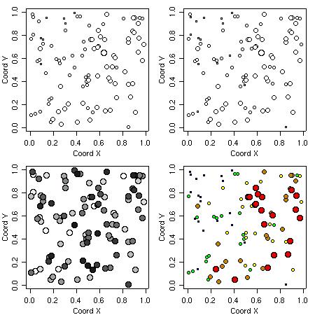
The function points.geodata produces a plot showing the data locations. Alternatively, points indicating the data locations can be added to a current plot.
There are options to specify point sizes, patterns and colors, which can be set to be proportional to the data values or specified quantiles.
Some examples of graphical outputs are illustrated by the commands and corresponding plots as shown below.
We start saving the current graphical parameters.
par.ori <- par(no.readonly = TRUE)
par(mfrow = c(2,2))
points(s100, xlab = "Coord X", ylab = "Coord Y")
points(s100, xlab = "Coord X", ylab = "Coord Y", pt.divide = "rank.prop")
points(s100, xlab = "Coord X", ylab = "Coord Y", cex.max = 1.7,
       col = gray(seq(1, 0.1, l=100)), pt.divide = "equal")
points(s100, pt.divide = "quintile", xlab = "Coord X", ylab = "Coord Y")
par(par.ori)
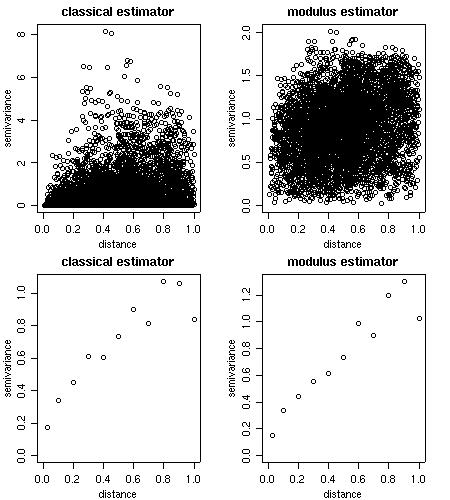
Empirical variograms are calculated using the function variog. There are options for the classical or modulus estimator.
Results can be returned as variogram clouds, binned or smoothed variograms.
cloud1 <- variog(s100, option = "cloud", max.dist=1)
cloud2 <- variog(s100, option = "cloud", estimator.type = "modulus", max.dist=1)
bin1 <- variog(s100, uvec=seq(0,1,l=11))
bin2  <- variog(s100, uvec=seq(0,1,l=11), estimator.type= "modulus")

par(mfrow=c(2,2))
plot(cloud1, main = "classical estimator")
plot(cloud2, main = "modulus estimator")
plot(bin1, main = "classical estimator")
plot(bin2, main = "modulus estimator")
par(par.ori)
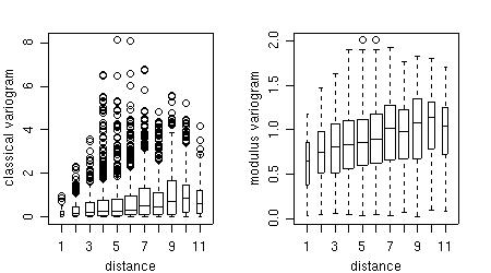
Furthermore, the points of the variogram clouds can be grouped into classes of distances ("bins") and displayed with a box-plot for each bin.
bin1 <- variog(s100,uvec = seq(0,1,l=11), bin.cloud = T)
bin2 <- variog(s100,uvec = seq(0,1,l=11), estimator.type = "modulus", bin.cloud = T)

par(mfrow = c(1,2))
plot(bin1, bin.cloud = T, main = "classical estimator")
plot(bin2, bin.cloud = T, main = "modulus estimator")
par(par.ori)
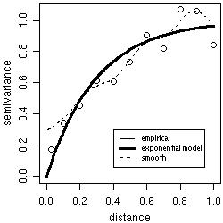
Theoretical and empirical variograms can be plotted and visually compared. For example, the figure below shows the theoretical variogram model used to simulate the data s100 and two estimated variograms.
bin1 <- variog(s100, uvec = seq(0,1,l=11))
plot(bin1)
lines.variomodel(cov.model = "exp", cov.pars = c(1,0.3), nugget = 0, max.dist = 1,  lwd = 3)
smooth <- variog(s100, option = "smooth", max.dist = 1, n.points = 100, kernel = "normal", band = 0.2)
lines(smooth, type ="l", lty = 2)
legend(0.4, 0.3, c("empirical", "exponential model", "smoothed"), lty = c(1,1,2), lwd = c(1,3,1))
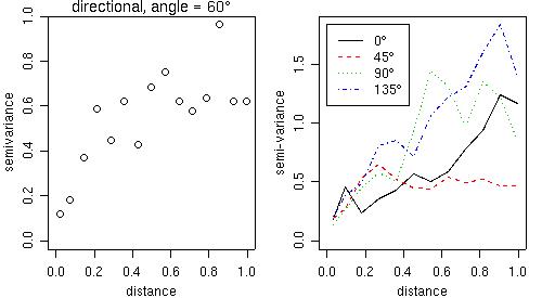
Directional variograms can also be computed by the function variog using the arguments direction and tolerance. For example, to compute a variogram for the direction 60 degrees with the default tolerance angle (22.5 degrees) the command would be:
vario60 <- variog(s100, max.dist = 1, direction=pi/3)
plot(vario60)
title(main = expression(paste("directional, angle = ", 60 * degree)))
and the plot is shown on the left panel of the figure below.
For a quick computation in four directions we can use the function variog4 and the corresponding plot is shown on the right panel of the next figure.
vario.4 <- variog4(s100, max.dist = 1)
plot(vario.4, lwd=2)
- by "eye": trying different models over empirical variograms (using the function lines.variomodel),
- by least squares fit of empirical variograms: with options for ordinary (OLS) and weighted (WLS) least squares (using the function variofit),
- by likelihood based methods: with options for maximum likelihood (ML) and restricted maximum likelihood (REML) (using the function likfit),
- Bayesian methods are also implemented and will be presented in Section 5 (using the function krige.bayes).
plot(variog(s100, max.dist=1))
lines.variomodel(cov.model="exp", cov.pars=c(1,.3), nug=0, max.dist=1)
lines.variomodel(cov.model="mat", cov.pars=c(.85,.2), nug=0.1, kappa=1,max.dist=1, lty=2)
lines.variomodel(cov.model="sph", cov.pars=c(.8,.8), nug=0.1,max.dist=1, lwd=2)
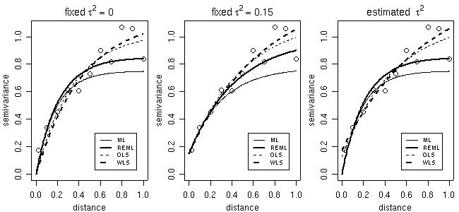
In the parameter estimation functions variofit and likfitthe nugget effect parameter can either be estimated or set to a fixed value. The same applies for smoothness, anisotropy and transformation parameters. Options for taking trends into account are also included. Trends can be specified as polynomial functions of the coordinates and/or linear functions of given covariates.
The commands below shows models fitted by different methods with options for fixed or estimated nugget parameter. Features not illustrated here include estimation of trends, anisotropy, smoothness and Box-Cox transformation parameter.
# Fitting models with nugget fixed to zero
ml <- likfit(s100, ini = c(1,0.5), fix.nugget = T)
reml <- likfit(s100, ini = c(1,0.5), fix.nugget = T, method = "RML")
ols <- variofit(bin1, ini = c(1,0.5), fix.nugget = T, weights="equal")
wls <- variofit(bin1, ini = c(1,0.5), fix.nugget = T)

# Fitting models with a fixed value for the nugget
ml.fn <- likfit(s100, ini = c(1,0.5), fix.nugget = T, nugget = 0.15)
reml.fn <- likfit(s100, ini = c(1,0.5), fix.nugget = T, nugget = 0.15, method = "RML")
ols.fn <- variofit(bin1,ini = c(1,0.5), fix.nugget = T, nugget = 0.15, weights="equal")
wls.fn <- variofit(bin1, ini = c(1,0.5), fix.nugget = T, nugget = 0.15)

# Fitting models estimated nugget
ml.n <- likfit(s100, ini = c(1,0.5), nug = 0.5)
reml.n <- likfit(s100, ini = c(1,0.5), nug = 0.5, method = "RML")
ols.n <- variofit(bin1, ini = c(1,0.5), nugget=0.5, weights="equal")
wls.n <- variofit(bin1, ini = c(1,0.5), nugget=0.5)

# Now, plotting fitted models against empirical variogram
par(mfrow = c(1,3))
plot(bin1, main = expression(paste("fixed ", tau^2 == 0)))
lines(ml, max.dist = 1)
lines(reml, lwd = 2, max.dist = 1)
lines(ols, lty = 2, max.dist = 1)
lines(wls, lty = 2, lwd = 2, max.dist = 1)
legend(0.5, 0.3, legend=c("ML","REML","OLS","WLS"),lty=c(1,1,2,2),lwd=c(1,2,1,2), cex=0.7)

plot(bin1, main = expression(paste("fixed ", tau^2 == 0.15)))
lines(ml.fn, max.dist = 1)
lines(reml.fn, lwd = 2, max.dist = 1)
lines(ols.fn, lty = 2, max.dist = 1)
lines(wls.fn, lty = 2, lwd = 2, max.dist = 1)
legend(0.5, 0.3, legend=c("ML","REML","OLS","WLS"), lty=c(1,1,2,2), lwd=c(1,2,1,2), cex=0.7)

plot(bin1, main = expression(paste("estimated  ", tau^2)))
lines(ml.n, max.dist = 1)
lines(reml.n, lwd = 2, max.dist = 1)
lines(ols.n, lty = 2, max.dist = 1)
lines(wls.n, lty =2, lwd = 2, max.dist = 1)
legend(0.5, 0.3, legend=c("ML","REML","OLS","WLS"), lty=c(1,1,2,2), lwd=c(1,2,1,2), cex=0.7)

par(par.ori)
Summary methods have been written to summarize the resulting objects.
For example, for the model with estimated nugget fitted by maximum likelihood, typing:
ml.n
will produce the output:likfit: estimated model parameters: beta tausq sigmasq phi 0.7766 0.0000 0.7517 0.1827 likfit: maximised log-likelihood = -83.5696whilst a more detailed summary is obtained with:
> summary(ml.n)
Summary of the parameter estimation
-----------------------------------
Estimation method: maximum likelihood

Parameters of the mean component (trend):
  beta
0.7766

Parameters of the spatial component:
   correlation function: exponential
      (estimated) variance parameter sigmasq (partial sill) =  0.7517
      (estimated) cor. fct. parameter phi (range parameter)  =  0.1827
   anisotropy parameters:
      (fixed) anisotropy angle = 0  ( 0 degrees )
      (fixed) anisotropy ratio = 1

Parameter of the error component:
      (estimated) nugget =  0

Transformation parameter:
      (fixed) Box-Cox parameter = 1 (no transformation)

Maximised Likelihood:
   log.L n.params      AIC      BIC
-83.5696   4.0000 175.1391 185.5598

Call:
likfit(geodata = s100, ini.cov.pars = c(1, 0.5), nugget = 0.5)
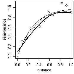
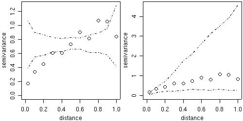
Two kinds of variogram envelopes
computed by simulation are
illustrated in the figure below.
The plot on the left-hand side shows an envelope based on
permutations of the data values across the locations,
i.e. envelopes built under
the assumption of no spatial correlation.
The envelopes shown on the right-hand side are based on
simulations from a given set of model parameters, in this example the parameter
estimates from the WLS variogram fit.
This envelope shows the variability of the empirical variogram.
env.mc <- variog.mc.env(s100, obj.var=bin1)
env.model <- variog.model.env(s100, obj.var=bin1, model=wls)

par(mfrow=c(1,2))
plot(bin1, envelope=env.mc)
plot(bin1, envelope=env.model)
par(par.ori)
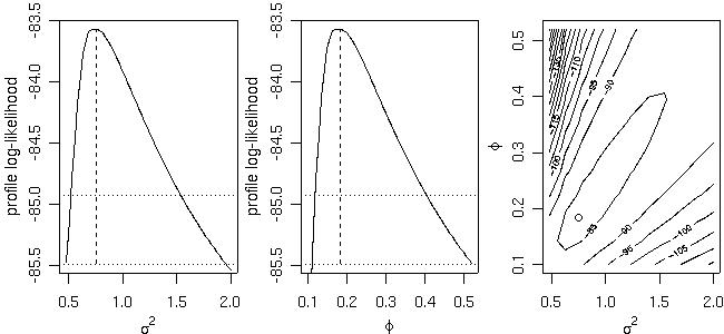
Profile likelihoods (1-D and 2-D) are computed by the function proflik. Here we show the profile likelihoods for the covariance parameters of the model without nugget effect previously fitted by likfit.
WARNING: RUNNING THE NEXT COMMAND CAN BE TIME-CONSUMING
prof <- proflik(ml, geodata = s100, sill.val = seq(0.48, 2, l=11),
		range.val = seq(0.1, 0.52, l=11), uni.only = FALSE)

par(mfrow=c(1,3))
plot(prof, nlevels=16)
par(par.ori)
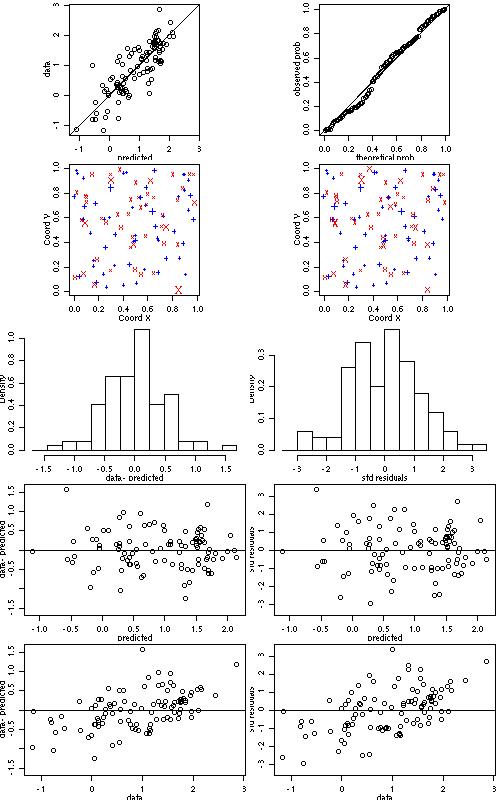
xv.ml <- xvalid(s100, model=ml)
xv.wls <- xvalid(s100, model=wls)
WARNING: RUNNING THE NEXT COMMAND CAN BE TIME-CONSUMING
xvR.ml <- xvalid(s100, model=ml, reest=TRUE)
xvR.wls <- xvalid(s100, model=wls, reest=TRUE, variog.obj=bin1)

par(mfcol = c(5,2), mar=c(3,3,.5,.5), mgp=c(1.5,.7,0))
plot(xv.wls)
par(par.ori)
- Simple kriging
- Ordinary kriging
- Trend (universal) kriging
- External trend kriging
There are additional options for Box-Cox transformation (and back transformation of the results) and anisotropic models.
Simulations can be drawn from the resulting predictive
distributions if requested.
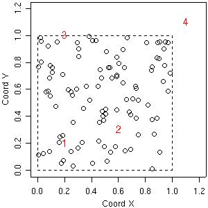
As a first example consider the prediction at four locations labeled 1, 2, 3, 4 and indicated in the figure below.
plot(s100$coords, xlim=c(0,1.2), ylim=c(0,1.2), xlab="Coord X", ylab="Coord Y")
loci <- matrix(c(0.2, 0.6, 0.2, 1.1, 0.2, 0.3, 1.0, 1.1), ncol=2)
text(loci, as.character(1:4), col="red")
polygon(x=c(0,1,1,0), y=c(0,0,1,1), lty=2)
The command to perform ordinary kriging using the parameters estimated by weighted least squares with nugget fixed to zero would be:
kc4 <- krige.conv(s100, locations = loci, krige = krige.control(obj.m = wls))
The output is a list including the predicted values (kc4$predict) and the kriging variances (kc4$krige.var).
Consider now a second example. The goal is to perform prediction on a grid covering the area and to display the results. Again, we use ordinary kriging. The commands are:
# defining the grid
pred.grid <-  expand.grid(seq(0,1, l=51), seq(0,1, l=51))
# kriging calculations
kc <- krige.conv(s100, loc = pred.grid, krige = krige.control(obj.m = ml))
# displaying predicted values
image(kc, loc = pred.grid, col=gray(seq(1,0.1,l=30)), xlab="Coord X", ylab="Coord Y")
As an example consider a model without nugget and including uncertainty in the mean, sill and range parameters. Prediction at the four locations indicated above is performed by typing a command like:
WARNING: RUNNING THE NEXT COMMAND CAN BE TIME-CONSUMINGbsp4 <- krige.bayes(s100, loc = loci, prior = prior.control(phi.discrete = seq(0,5,l=101), phi.prior="rec"), output=output.control(n.post=5000))
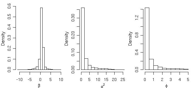
Histograms showing posterior distribution for the model parameters can be plotted by typing:
par(mfrow=c(1,3), mar=c(3,3,.5,.5), mgp=c(2,1,0))
hist(bsp4$posterior$sample$beta, main="", xlab=expression(beta), prob=T)
hist(bsp4$posterior$sample$sigmasq, main="", xlab=expression(sigma^2), prob=T)
hist(bsp4$posterior$sample$phi, main="", xlab=expression(phi), prob=T)
par(par.ori)
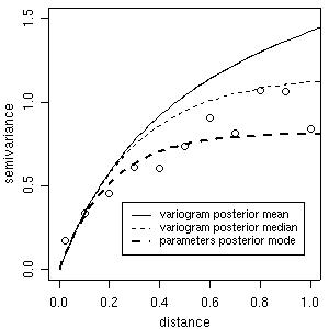
Using summaries of these posterior distributions (means, medians or modes) we can check the "estimated Bayesian variograms" against the empirical variogram, as shown in the next figure. Notice that it is also possible to compare these estimates with other fitted variograms such as the ones computed in Section 3.
plot(bin1, ylim = c(0,1.5))
lines(bsp4, max.dist = 1.2, summ = mean)
lines(bsp4, max.dist = 1.2, summ = median, lty = 2)
lines(bsp4, max.dist = 1.2, summ = "mode", post="par",lwd = 2, lty = 2)
legend(0.25, 0.4, legend = c("variogram posterior mean", "variogram posterior median", "parameters posterior mode"), lty = c(1,2,2), lwd = c(1,1,2), cex = 0.8)
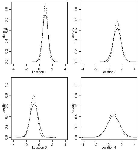
The next figure shows predictive distributions at the four selected locations.
Dashed lines show Gaussian distributions with mean and variance given by results of ordinary kriging obtained
in Section 4.
The full lines correspond to the Bayesian prediction. The plot shows results of density estimation
using samples from the predictive distributions.
par(mfrow=c(2,2), mar=c(3,3,.5,.5), mgp=c(1.5,.7,0))
   for(i in 1:4){
        kpx <- seq(kc4$pred[i] - 3*sqrt(kc4$krige.var[i]), kc4$pred[i] +3*sqrt(kc4$krige.var[i]), l=100)
	kpy <- dnorm(kpx, mean=kc4$pred[i], sd=sqrt(kc4$krige.var[i]))
	bp <- density(bsp4$predic$sim[i,])
	rx <- range(c(kpx, bp$x))
	ry <- range(c(kpy, bp$y))
	plot(cbind(rx, ry), type="n", xlab=paste("Location", i), ylab="density", xlim=c(-4, 4), ylim=c(0,1.1))
	lines(kpx, kpy, lty=2)
	lines(bp)
   }
par(par.ori)
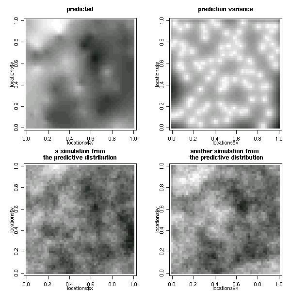
Consider now, under the same model assumptions, obtaining simulations from the predictive distributions on a grid of points covering the area. The commands to define the grid and perform Bayesian prediction are:
pred.grid <- expand.grid(seq(0,1, l=31), seq(0,1, l=31))WARNING: RUNNING THE NEXT COMMAND CAN BE TIME-CONSUMING
bsp <- krige.bayes(s100, loc = pred.grid, prior = prior.control(phi.discrete = seq(0,5,l=51)),
                   output=output.control(n.predictive=2))
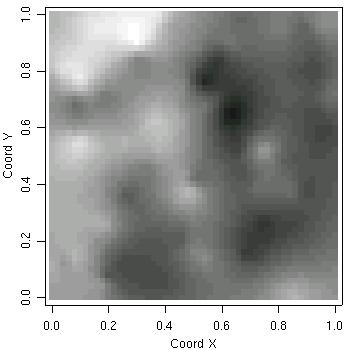
Maps with the summaries and simulations of the predictive distribution can be plotted as follows.
par(mfrow=c(2,2))
image(bsp, loc = pred.grid, main = "predicted", col=gray(seq(1,0.1,l=30)))
image(bsp, val ="variance", loc = pred.grid,
      main = "prediction variance", col=gray(seq(1,0.1,l=30)))
image(bsp, val = "simulation", number.col = 1, loc = pred.grid,
      main = "a simulation from\nthe predictive distribution", col=gray(seq(1,0.1,l=30)))
image(bsp, val = "simulation", number.col = 2,loc = pred.grid,
      main = "another simulation from \n the predictive distribution", col=gray(seq(1,0.1,l=30)))
par(par.ori)
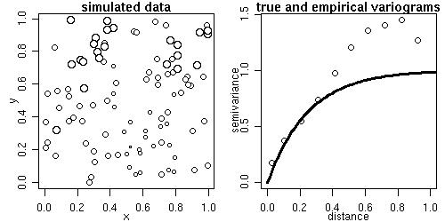
The function grf generates simulations of Gaussian random fields on regular or irregular sets of locations
Some of its functionality is illustrated by the next commands.
sim1 <- grf(100, cov.pars=c(1, .25))
points.geodata(sim1, main="simulated locations and values")
plot(sim1, max.dist=1, main="true and empirical variograms")
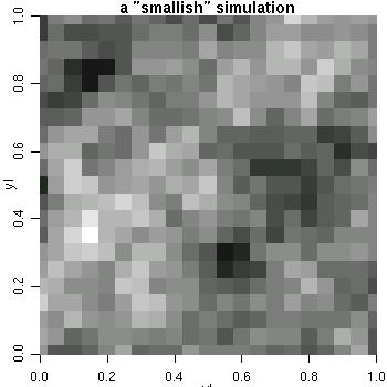
sim2 <- grf(441, grid="reg", cov.pars=c(1, .25))
image(sim2, main="a small-ish simulation", col=gray(seq(1, .1, l=30)))
sim3 <- grf(40401, grid="reg", cov.pars=c(10, .2), met="circ")
image(sim3, main="simulation on a fine grid", col=gray(seq(1, .1, l=30)))
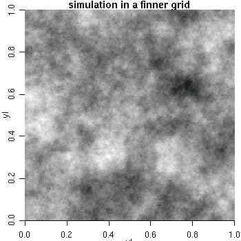
NOTE: we recommend the package RandomFields for a more comprehensive implementation for simulation of Gaussian Random Fields.
 > cite.geoR()

 To cite geoR in publications, use

 RIBEIRO Jr., P.J. & DIGGLE, P.J. (2001) geoR: A package for
 geostatistical analysis. R-NEWS, Vol 1, No 2, 15-18. ISSN 1609-3631.

 Please cite geoR when using it for data analysis!

 A BibTeX entry for LaTeX users is

 @Article{,
     title         = {{geoR}: a package for geostatistical analysis},
     author        = {Ribeiro Jr., P.J. and Diggle, P.J.},
     journal       = {R-NEWS},
     year          = {2001},
     volume        = {1},
     number        = {2},
     pages         = {15--18},
     issn          = {1609-3631},
     url           = {http://cran.R-project.org/doc/Rnews}
 }