Introduction
To R

Reading In Data

If you have a bunch of numbers in a file, you can use the scan() function to read them into an R vector:

> x <- scan("file1.dat")

If the numbers are separated by, for example, a comma or a blank space, you need to inform scan() of this, otherwise numbers are assumed to be separated by newlines:

> x <- scan("file2.dat",sep=",")

You can also read in character data, but you need to tell scan() about it by using the what= argument:

> c1 <- scan('chars.dat',what='')
> c1
[1] "this"      "is"        "some"      "character" "data"

R reads each word into an element of the vector. If you want R to treat each line as an element, then you tell scan() that the separator is an end-of-line character, represented by \n:

> c2 <- scan("chars.dat",what='',sep='\n')
> c2
[1] "this is some"   "character data"

Simple Summary Statistics

R has the functions mean(), median(), min(), and max() which do the obvious things, as well as the summary() function mentioned earlier.

You can also compute the variance of a set of numbers with the var() function.

Random Number Generators

R can generate all sorts of random (strictly pseudo-random) numbers - uniform, normal, binomial etc. As well as the generator function each distribution has a function to compute the cumulative probability, density and quantiles. For example, the Normal distribution is represented by:

`rnorm(n,mean=0,sd=1)`	Generate `n` numbers
`dnorm(q,mean=0,sd=1)`	Density for `q`th quantile
`pnorm(q,mean=0,sd=1)`	Probability for `q`th quantile
`qnorm(p,mean=0,sd=1)`	Quantile for probability `p`

Histogramming some things

We can look at the output of rnorm() with the hist() function:

> hist(rnorm(1000))      mean 0, s.d.=1
> hist(rnorm(1000,2))    mean 2, s.d.=1
> hist(rnorm(1000,2,2))  mean 2, s.d.=2

Or for more variety, random numbers from chi-squared distributions with varying degrees of freedom:

> hist(rchisq(1000,df=2))
> hist(rchisq(1000,5))      df is required arg
> hist(rchisq(1000,100))

A Quick Quantile Query

Lets generate 10,000 numbers from a chi-squared distribution and see how close our numbers are to the theoretical 0.95% chi-squared quantiles:

> xch <- rchisq(10000,df=2)  lots of numbers
> qchisq(0.95,2)             whats the 95% quantile...
[1] 5.991465
> sum(xch < qchisq(.95,2))/length(xch)   what fraction of our data
                                       is under this....
[1] 0.9491

...which seems close enough to 0.95.

Time for a t-test

I have some data from a cloud seeding experiment. Scientists spray clouds with Silver Iodide crystals and measure the rainfall. Then they dont spray Silver Iodide and measure the rainfall.

BUT Does it make any difference?

To get the data click on the links, save the data, and change the paths in the examples to find the files.

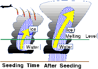
Rainfall for seeded clouds

Rainfall for unseeded clouds

Reading the data

We can just use the scan() function to read the data files into two vectors:

> unseeded <- scan("unseeded")
Read 26 items
> seeded <- scan("seeded")
Read 26 items

Looking at the data

We can histogram the data for a quick look:

> par(mfrow=c(2,1))  get both plots on
> hist(seeded)
> hist(unseeded)

This shows us how skew the numbers are. Perhaps we can make them look more normal with a log-transform:

> hist(log(seeded))
> hist(log(unseeded))

Yup, thats much nicer. We should use the log-transformed data in the analysis.

The t-test

Now we want to know whether could seeding significantly affects rainfall, i.e. whether one set of numbers is larger or smaller than the other. The t-test is used to test for the mean of two sets of numbers being equal. You compute the t-statistic, which is given by this formula:

The denominator is computed with:

where

Where and are the means of the two sets of numbers, and are the square-roots of the variances of the two sets, and and are the number of points in each data set.

Your Mission..

To compute the t-statistic for the log-transformed cloud-seeding data... Compute S first, then the SE12, then t. You will need the functions mean(), var() and length()

Click here for the solution.

The t-test in R

Now we have the t-statistic for those data. But what use is that? Well, we can look it up in a table and see if that tells us if the difference in the means of the seeded and unseeded data is significant. We can also calculate a 95% confidence interval of the difference in the means, and see if this excludes zero. The easiest thing to do, however, is to get R to do all this for us:

> t.test(log(seeded),log(unseeded),var.equal=T)
 
        Two Sample t-test
 
data:  log(seeded) and log(unseeded) 
t = 2.5444, df = 50, p-value = 0.01408 
alternative hypothesis: true difference in means is not equal to 0 
95 percent confidence interval:
 0.2408650 2.0466972 
sample estimates:
mean of x mean of y 
 5.134187  3.990406

Note how it computes the t value - this should be the same as what we computed it to be the long way...

The interesting thing here is the 95 percent confidence interval - this tells us that the difference in means is significantly not zero - which then tells us that maybe the cloud seeding is doing something.

Contents