Radial Plot for a Compact Letter Display Vector

This function does a radial plot based on the vector of letters resulted from pairwise comparisons.

radial_cld(cld, labels = cld, col = NULL, means = NULL,
  perim = FALSE, legend = TRUE)

Arguments

cld	Character vector with strings of letters that indicates which pair of treatment cells are not different.
labels	Vector of text to be annotated next each point.
col	Vector of colors to be used in the segments that joint points.
means	Numeric vector with the estimated means of treatment cells. It is used to place points at distances proportional to the differences on means.
perim	Logical value (default is FALSE) that indicates weather draw or not a circle in the perimeter passing by the points.
legend	Logical value (default is TRUE) that indicates weather daraw or not the legend.

Value

None is returned, only the plot is done.

See also

cld2().

Examples

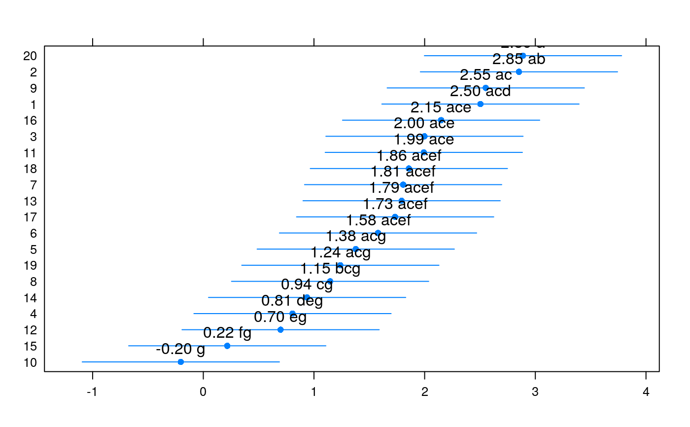
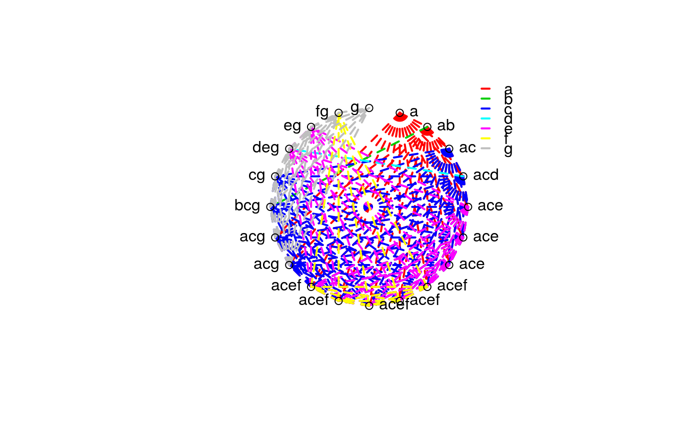
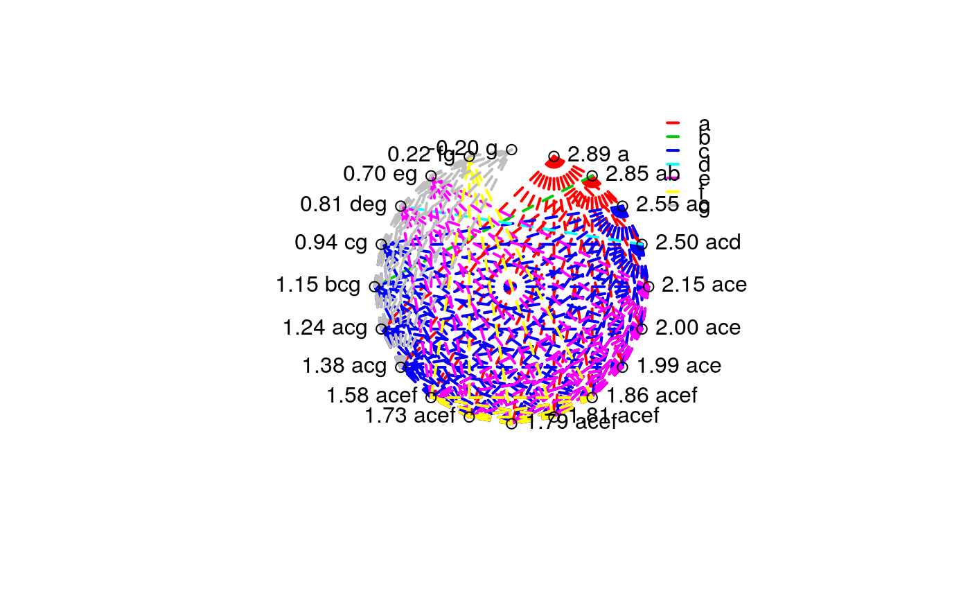
set.seed(4321)
td <- data.frame(trt = rep(sample(1:20), each = 5))
td$y <- rnorm(nrow(td), mean = 0.15 * sort(td$trt), sd = 1)

plot(y ~ trt, data = td)

# Fit the model.
td$trt <- factor(td$trt)
m0 <- lm(y ~ trt, data = td)
anova(m0)
#> Analysis of Variance Table
#> 
#> Response: y
#>           Df Sum Sq Mean Sq F value    Pr(>F)    
#> trt       19 65.815  3.4640  3.4576 5.194e-05 ***
#> Residuals 80 80.146  1.0018                      
#> ---
#> Signif. codes:  0 ‘***’ 0.001 ‘**’ 0.01 ‘*’ 0.05 ‘.’ 0.1 ‘ ’ 1
summary(m0)
#> 
#> Call:
#> lm(formula = y ~ trt, data = td)
#> 
#> Residuals:
#>     Min      1Q  Median      3Q     Max 
#> -2.0226 -0.6637  0.0693  0.6348  2.2642 
#> 
#> Coefficients:
#>             Estimate Std. Error t value Pr(>|t|)    
#> (Intercept)  2.50426    0.44762   5.595 2.99e-07 ***
#> trt2         0.34782    0.63303   0.549 0.584225    
#> trt3        -0.50600    0.63303  -0.799 0.426472    
#> trt4        -1.69826    0.63303  -2.683 0.008870 ** 
#> trt5        -1.12692    0.63303  -1.780 0.078841 .  
#> trt6        -0.92557    0.63303  -1.462 0.147624    
#> trt7        -0.69882    0.63303  -1.104 0.272939    
#> trt8        -1.35856    0.63303  -2.146 0.034894 *  
#> trt9         0.04789    0.63303   0.076 0.939889    
#> trt10       -2.70744    0.63303  -4.277 5.20e-05 ***
#> trt11       -0.51198    0.63303  -0.809 0.421043    
#> trt12       -1.80581    0.63303  -2.853 0.005517 ** 
#> trt13       -0.71239    0.63303  -1.125 0.263802    
#> trt14       -1.56631    0.63303  -2.474 0.015465 *  
#> trt15       -2.28781    0.63303  -3.614 0.000525 ***
#> trt16       -0.35552    0.63303  -0.562 0.575952    
#> trt17       -0.77093    0.63303  -1.218 0.226867    
#> trt18       -0.64693    0.63303  -1.022 0.309886    
#> trt19       -1.26594    0.63303  -2.000 0.048916 *  
#> trt20        0.38425    0.63303   0.607 0.545568    
#> ---
#> Signif. codes:  0 ‘***’ 0.001 ‘**’ 0.01 ‘*’ 0.05 ‘.’ 0.1 ‘ ’ 1
#> 
#> Residual standard error: 1.001 on 80 degrees of freedom
#> Multiple R-squared:  0.4509,	Adjusted R-squared:  0.3205 
#> F-statistic: 3.458 on 19 and 80 DF,  p-value: 5.194e-05
#> 

library(multcomp)
library(doBy)

X <- LE_matrix(m0, effect = "trt")
rownames(X) <- levels(td$trt)

ci <- apmc(X, m0, focus = "trt", test = "fdr")
ci$cld <- with(ci, ordered_cld(cld, fit))
ci <- ci[order(ci$fit, decreasing = TRUE), ]

library(latticeExtra)

segplot(reorder(trt, fit) ~ lwr + upr,
        centers = fit,
        data = ci,
        draw = FALSE,
        cld = ci$cld) +
    layer(panel.text(x = centers,
                     y = z,
                     labels = sprintf("%0.2f %s",
                                      centers,
                                      cld),
                     pos = 3))

radial_cld(cld = ci$cld)
#> Warning: Length of vector `col` is different of the number of unique letters. Colors will be recycled.
radial_cld(cld = ci$cld, means = ci$fit, perim = TRUE)
#> Warning: Length of vector `col` is different of the number of unique letters. Colors will be recycled.
radial_cld(cld = ci$cld, col = 1:3)
#> Warning: Length of vector `col` is different of the number of unique letters. Colors will be recycled.
radial_cld(cld = ci$cld, col = 1:3)
#> Warning: Length of vector `col` is different of the number of unique letters. Colors will be recycled.
radial_cld(cld = ci$cld, labels = sprintf("%0.2f %s", ci$fit, ci$cld))
#> Warning: Length of vector `col` is different of the number of unique letters. Colors will be recycled.