|
|
A quick summary for the geodata object can be obtained using a method for summary which will return a information on the coordinates and data values.
The elements of the list $covariate, $borders and/or units.m will be also summarized if present in the geodata object.
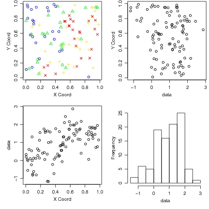
The function plot.geodata shows a 2 × 2 display with data locations (top plots) and data versus coordinates (bottom plots). For an object of the class geodata the command plot(s100) produce the output shown in Figure 3.1.
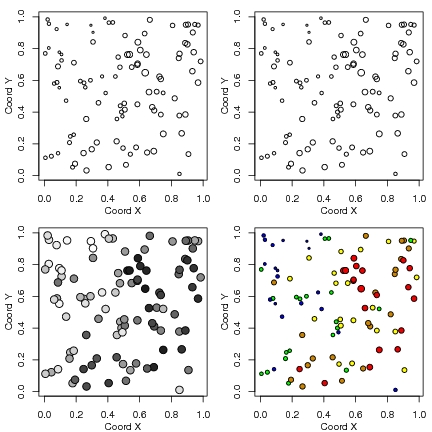
The function points.geodata produces a plot showing the data locations. Alternatively, points indicating the data locations can be added to a current plot. There are options to specify point sizes, patterns and colors, which can be set to be proportional to the data values or specified quantiles. Some examples of graphical outputs are illustrated by the commands below and corresponding plots as shown in Figure 3.1.
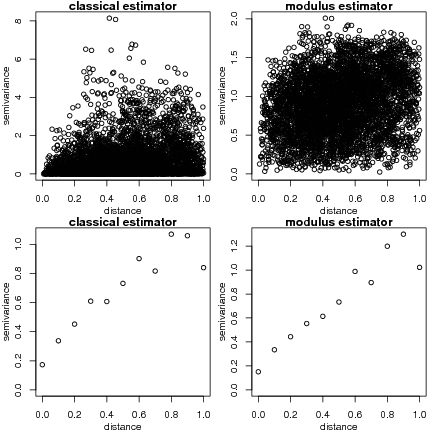
Empirical variograms are calculated using the function variog. There are options for the classical or modulus estimator. Results can be returned as variogram clouds, binned or smoothed variograms. There are methods for plot to facilitate the display of the results as shown in Figure 3.
Several results are returned by the function variog. The first three are the more important ones and contains the distances, the estimated semivariance and the number of pairs for each bin.
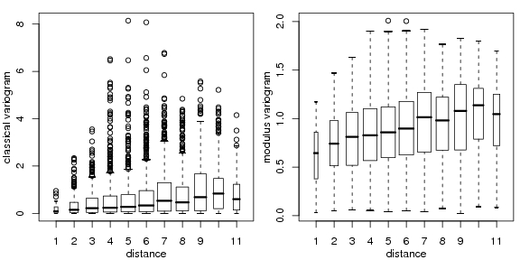
Furthermore, the points of the variogram clouds can be grouped into classes of distances ("bins") and displayed with a box-plot for each bin as shown in Figure 3.2. This can be used as an exploratory tool to access variogram results.
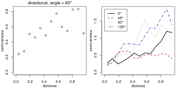
Directional variograms can also be computed by the function variog using the arguments ‘direction’ and ‘tolerance’. For example, to compute a variogram for the direction 60 degrees with the default tolerance angle (22.5 degrees) the command would be:
For a quick computation in four directions we can use the function variog4 which by default computes variogram for the direction angles 0o, 45o, 90o and 135o.
The Figure 5 show the directional variograms obtained with the commands above.
|
> par(mfrow = c(1, 2), mar = c(3, 3, 1.5, 0.5)) > plot(vario60) > title(main = expression(paste("directional, angle = ", + 60 * degree))) > plot(vario.4, lwd = 2)
|