Conventional geostatistical spatial interpolation (kriging) can be performed with options for:
There are additional options for Box-Cox transformation (and back transformation of the results) and anisotropic models. Simulations can be drawn from the resulting predictive distributions if requested.
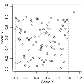
As a first example consider the prediction at four locations labeled 1, 2, 3, 4 and indicated in the figure below.
The command to perform ordinary kriging using the parameters estimated by weighted least squares with nugget fixed to zero would be:
The output is a list including the predicted values (kc4$predict) and the kriging variances (kc4$krige.var).
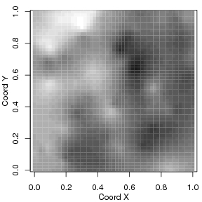
Consider now a second example. The goal is to perform prediction on a grid covering the area and to display the results. Again, we use ordinary kriging. The commands commands below defines a grid of locations and performs the prediction at those locations.
A method for the function image can be used for displaying predicted values as shown in the next Figure, as well as other prediction results returned by krige.conv.