Anthropometric measures: Bivariate continuous data
Source:vignettes/Weight_height.Rmd
Weight_height.RmdAbstract
The mglm4twin package implements multivariate
generalized linear models for twin and family data as proposed by Bonat
and Hjelmborg (2020). The core fit function mglm4twin is
employed for fitting a set of models. In this introductory vignette we
restrict ourselves to model bivariate continuous outcomes. We present a
set of special specifications of the standard ACE for continuous trait
in the context of twin data. This vignette reproduces the data analysis
presented in the Section 5.4 Dataset 4: Bivariate continuous data of
Bonat and Hjelmborg (2020).
Install and loading the mglm4twin package
To install the stable version of mglm4twin,
use devtools::install_git(). For more information, visit mglm4twin/README.
library(devtools)
install_git("bonatwagner/mglm4twin")
library(mglm4twin)
packageVersion("mglm4twin")
#> [1] '0.5.0'

require(mvtnorm)
Data set
The dataset anthro contains anthropometric measures
(weight and height) on 861 (327 DZ and 534 MZ) twin-pairs. The data set
is available as an example in the OpenMx package (Neale et al., 2016).
The main goal of this example is to illustrate how to deal with a fairly
common case of bivariate continuous traits in the context of twin
studies. Furthermore, we explore the flexibility of our proposed model
class and model the dispersion components as a linear combination of a
covariate of interest.
data(anthro)
head(anthro)
#>   weight height age Group Twin Twin_pair
#> 1     62 1.6499  24    DZ  535         1
#> 2     55 1.6299  24    DZ  535         2
#> 3     66 1.6599  20    DZ  536         1
#> 4     73 1.7000  20    DZ  536         2
#> 5     51 1.7300  20    DZ  537         1
#> 6     44 1.5698  20    DZ  537         2

## Standardize
anthro$age <- (anthro$age - mean(anthro$age))/sd(anthro$age)
anthro$weight <- (anthro$weight - mean(anthro$weight))/sd(anthro$weight)
anthro$height <- (anthro$height - mean(anthro$height))/sd(anthro$height)
Model specification
The model specification is done in three steps:
- Specifying the linear predictor (mean model).
- Specifying the matrix linear predictor (twin dependence struture).
- Specifying link and variance function suitable to be response variable type.
Specyfing the linear predictor
In the anthro data set we have three covariates available for composing the linear predictor. Thus, the linear predictor is given by
form_Wt <- weight ~ age + Group*Twin_pair
form_Ht <- height ~ age + Group*Twin_pair
Specyfing the matrix linear predictor
In this example, we are going to specify and fit only the two models presented in Table 5 of Bonat and Hjelmborg (2020). The first model is an specification of the ACE model where all dispersion components are modelled as a function of the covariate age. The second is a special case of the former whre all non-significant terms were excluded.
## ACE model
biv0 <- list("formE1" = ~ age, "formE2" = ~ age, "formE12" = ~ age,
             "formA1" = ~ age, "formA2" = ~ age, "formA12" = ~ age,
             "formC1" = ~ age, "formC2" = ~ age, "formC12" = ~ age)
Z_biv0 <- mt_twin(N_DZ = 327, N_MZ = 534, n_resp = 2, model = "ACE",
                    formula = biv0, data = anthro)

## Special case of ACE model
biv4 <- list("formE1" = ~ age, "formE2" = ~ age, "formE12" = ~ 1,
             "formA1" = ~ age, "formA2" = ~ 1, "formA12" = ~ 1)
Z_biv4 <- mt_twin(N_DZ = 327, N_MZ = 534, n_resp = 2, model = "AE",
                  formula = biv4, data = anthro)
Model fitting
The main fitting function in the mglm4twin package is
the mglm4twin() function. it was designed to be similar to
standard model fitting functions in R such as
lm() and glm().
## Initial values
control_initial <- list()
control_initial$regression <- list("R1" = c(0.13, 0.10, -0.20, -0.02, 0.037),
                                   "R2" = c(0.23, 0.01, -0.27, -0.11, 0.11))
control_initial$power <- list(c(0), c(0))
control_initial$tau <- c(0.15, 0, 0.12, rep(0,15))

fit_0 <- mglm4twin(linear_pred = c(form_Wt, form_Ht), matrix_pred = Z_biv0,
                          control_initial = control_initial,
                          control_algorithm = list(tuning = 0.5),
                          power_fixed = c(TRUE, TRUE),
                          data = anthro)

control_initial$tau <- c(0.15, 0, 0.12, rep(0,6))
fit_4 <- mglm4twin(linear_pred = c(form_Wt, form_Ht), matrix_pred = Z_biv4,
                   control_initial = control_initial,
                   control_algorithm = list(tuning = 0.5),
                   power_fixed = c(TRUE, TRUE),
                   data = anthro)
Model output
The mglm4twin package offers a general
summary() function that can be customized to show the
dispersion components (standard output) or measures of interest
(biometric = TRUE) as genetic correlation and
heritability.
Parameter estimates and standard errors
est0 <- aux_summary(fit_0, formula = biv0, type = "otimist", data = anthro)[,c(1,2,3,4)]
est4 <- aux_summary(fit_4, formula = biv4, type = "otimist", data = anthro)[,c(1,2,3,4)]
Table5 <- data.frame("Estimates" = est0$Estimates,
                     "Std.error" = est0$Std..Error,
                     "Z.value" = est0$Z.value,
                     "Estimates" = c(est4$Estimates[1:5], NA, est4$Estimates[6:8],
                                     NA,est4$Estimates[9], rep(NA, 7)),
                     "Std.error" = c(est4$Std..Error[1:5], NA, est4$Std..Error[6:8], NA,
                                     est4$Std..Error[9], rep(NA, 7)),
                     "Z.value" = c(est4$Z.value[1:5], NA, est4$Z.value[6:8], NA,
                                   est4$Z.value[9], rep(NA, 7)))
rownames(Table5) <- c("E1", "E1.age", "E2", "E2.age", "E12", "E12.age","A1","A1.age",
                      "A2", "A2.age", "A12", "A12.age", "C1", "C1.age", "C2", "C2.age",
                      "C12", "C12.age")
Table5 <- round(Table5, 2)
Reproducing Table 5 of Bonat and Hjelmborg (2020)
Table5
#>         Estimates Std.error Z.value Estimates.1 Std.error.1 Z.value.1
#> E1           0.15      0.01   16.09        0.16        0.01     16.18
#> E1.age       0.03      0.01    3.16        0.03        0.01      3.78
#> E2           0.12      0.01   16.17        0.12        0.01     16.26
#> E2.age       0.02      0.01    2.55        0.02        0.01      3.01
#> E12          0.02      0.01    3.62        0.02        0.01      3.97
#> E12.age      0.00      0.01   -0.27          NA          NA        NA
#> A1           0.96      0.10    9.86        0.85        0.04     20.53
#> A1.age       0.23      0.09    2.49        0.11        0.03      3.48
#> A2           0.90      0.09   10.32        0.88        0.04     21.48
#> A2.age       0.04      0.09    0.50          NA          NA        NA
#> A12          0.47      0.07    6.61        0.44        0.03     14.02
#> A12.age     -0.03      0.07   -0.42          NA          NA        NA
#> C1          -0.12      0.09   -1.34          NA          NA        NA
#> C1.age      -0.14      0.09   -1.64          NA          NA        NA
#> C2          -0.02      0.09   -0.21          NA          NA        NA
#> C2.age      -0.05      0.08   -0.55          NA          NA        NA
#> C12         -0.03      0.07   -0.41          NA          NA        NA
#> C12.age      0.02      0.07    0.29          NA          NA        NA
Reproducing Figure 6 of Bonat and Hjelmborg (2020)
Computing measures of interest, heritability, genetic and phenotipic correlations.
## Computing measures of interest
Age = seq(-1.90, 1.70, l = 100)
point <- fit_4$Covariance

# Heritability
h_wt <- (point[6] + point[7]*Age)/(point[1] + point[2]*Age + point[6] + point[7]*Age)
h_ht <- (point[8])/(point[3] + point[4]*Age + point[8])
h_ht_wt <- point[9]/(point[5] + point[9])

# Genetic and phenotipic correlation
r_G <- point[9]/(sqrt(point[6] + point[7]*Age)*sqrt(point[8]))
std_1 <- sqrt(point[1] + point[2]*Age + point[6] + point[7]*Age)
std_2 <- sqrt(point[3] + point[4]*Age + point[8])
r_P <- (point[9] + point[5])/(std_1*std_2)
Inference for complex models like the one in this example is quite challenging. Thus, we opted to perform inference based on simulation from the assymptotic distribution of the estimating function estimators.
require(mvtnorm)
Age = seq(-1.90, 1.70, l = 50)

# Point estimates
point1 <- fit_4$Covariance

# Covariance matrix (otimist - Gaussian case -> maximum likelihood estimator)
COV <- -2*fit_4$joint_inv_sensitivity[11:19, 11:19]

## Simulating from the assymptotic ditribution
point <- rmvnorm(n = 10000, mean = point1, sigma = as.matrix(COV))
res_h_wt <- matrix(NA, nrow = 50, ncol = 10000)
res_h_ht <- matrix(NA, nrow = 50, ncol = 10000)
res_ht_wt <- matrix(NA, nrow = 50, ncol = 10000)
res_r_G <- matrix(NA, nrow = 50, ncol = 10000)
res_r_P <- matrix(NA, nrow = 50, ncol = 10000)
res_r_E <- matrix(NA, nrow = 50, ncol = 10000)

for(i in 1:10000) {
  h_wt <- (point[i,6] + point[i,7]*Age)/(point[i,1] + point[i,2]*Age + point[i,6] + point[i,7]*Age)
  res_h_wt[,i] <- h_wt
  h_ht <- (point[i,8])/(point[i,3] + point[i,4]*Age + point[i,8])
  res_h_ht[,i] <- h_wt
  h_ht_wt <- point[i,9]/(point[i,5] + point[i,9])
  res_ht_wt[,i] <- h_ht_wt
  r_G <- point[i,9]/(sqrt(point[i,6] + point[i,7]*Age)*sqrt(point[i,8]))
  res_r_G[,i] <- r_G
  std_1 <- sqrt(point[i,1] + point[i,2]*Age + point[i,6] + point[i,7]*Age)
  std_2 <- sqrt(point[i,3] + point[i,4]*Age + point[i,8])
  r_P <- (point[9] + point[5])/(std_1*std_2)
  res_r_P[,i] <- r_P
  r_E <- point[i,5]/(sqrt(point[i,1] + point[i,2]*Age)*sqrt(point[i,3] + point[i,4]*Age))
  res_r_E[,i] <- r_E
}
Based on the simulated values is easy to get point estimates and confidence intervals for all measures of interest.
Estimates <- c(rowMeans(res_h_wt), rowMeans(res_h_ht),
               rowMeans(res_ht_wt),
               rowMeans(res_r_G), rowMeans(res_r_E),
               rowMeans(res_r_P))
Ic_Min <- c(apply(res_h_wt, 1, quantile, 0.025),
            apply(res_h_ht, 1, quantile, 0.025),
            apply(res_ht_wt, 1, quantile, 0.025),
            apply(res_r_G, 1, quantile, 0.025),
            apply(res_r_E, 1, quantile, 0.025),
            apply(res_r_P, 1, quantile, 0.025))
Ic_Max <- c(apply(res_h_wt, 1, quantile, 0.975),
            apply(res_h_ht, 1, quantile, 0.975),
            apply(res_ht_wt, 1, quantile, 0.975),
            apply(res_r_G, 1, quantile, 0.975),
            apply(res_r_E, 1, quantile, 0.975),
            apply(res_r_P, 1, quantile, 0.975))
data_graph <- data.frame("Estimates" = Estimates, "Ic_Min" = Ic_Min,
                         "Ic_Max" = Ic_Max, "Age" = rep(Age, 6),
                         "Parameter" = rep(c("h1","h2","h12","G","E","P"), each = 50))
Probably, the most effective way to show such a complex results is through a plot.
require(lattice)
#> Loading required package: lattice
require(latticeExtra)
#> Loading required package: latticeExtra
source("https://raw.githubusercontent.com/walmes/wzRfun/master/R/panel.cbH.R")
data_graph$Parameter <- factor(data_graph$Parameter,
                               levels = c("h1","h2","h12","G","E","P"))
levels(data_graph$Parameter) <- c("Weight heritability",
                                  "Height heritability",
                                  "Biv. heritability",
                                  "Genetic correlation",
                                  "Environmental correlation",
                                  "Phenotypic correlation")

ylim = list("1" = c(0.75,1), "1" = c(0.75, 1),
            "3" = c(0.75,1), "2" = c(0.1, 1),
            "3" = c(0.1,1), "3" = c(0.1, 1))

xy1 <- xyplot(Estimates ~ Age | Parameter, data = data_graph,
              ylim = ylim,
              type = "l", ly = data_graph$Ic_Min,
              xlab = c("Standardized age"),
              uy = data_graph$Ic_Max, scales = "free",
              cty = "bands", alpha = 0.25, prepanel = prepanel.cbH,
              panel = panel.cbH)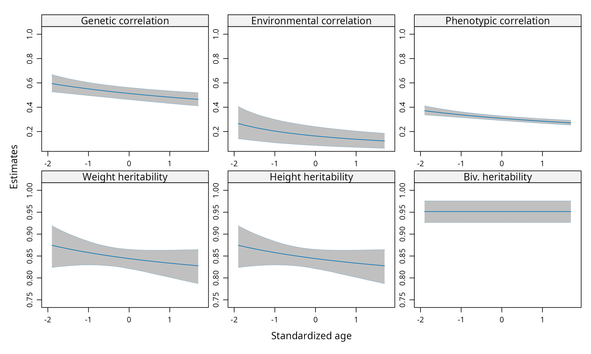
Genetic, environment and phenotypic correlations (first line). Body weight heritability, height heritability and bivariate heritability (second line) - Bivariate continuous Twin data.