Gaussian distribution with interval data
The following independent observations were taken from one r.v. \(X \sim N(\mu, \sigma^{2})\).
56.4, 54.2, 65.3, 49.2, 50.1, 56.9, 58.9, 62.5, 70, 61
another 5 observations are known to be less than 50.
it is known that 3 other observations are greater than 65.
Likelihood
Write the likelihood function.
The likelihood can be expressed as
\[ \begin{align*} L(\theta) &= \left( \prod_{i = 1}^{10} f(x_{i}) \right) \times (F(50))^{5} \times (1 - F(65))^{3}\\ &= \left( \prod_{i = 1}^{10} \phi \left( \frac{y_{i} - \mu}{\sigma} \right) \right) \times \left( \Phi \left( \frac{50 - \mu}{\sigma} \right) \right)^{5} \times \left( 1 - \Phi \left( \frac{65 - \mu}{\sigma} \right) \right)^{3}\\ l(\theta) &= \sum_{i = 1}^{10} \log \phi \left( \frac{y_{i} - \mu}{\sigma} \right) + 5~\log \Phi \left( \frac{50 - \mu}{\sigma} \right) + 3~\log \left( 1 - \Phi \left( \frac{65 - \mu}{\sigma} \right) \right). \end{align*} \]
# likelihood ---------------------------------------------------------------------
## if logsigma = TRUE, we do the parametrization using log(sigma)
lkl.norm <- function(par, xs, less.than, more.than, logsigma = FALSE) {
    if (logsigma) par[2] <- exp(par[2])
    l1 <- sum(dnorm(xs, mean = par[1], sd = par[2], log = TRUE))
    l2 <- 5 * log(pnorm(less.than, mean = par[1], sd = par[2]))
    l3 <- 3 * log(1 - pnorm(more.than, mean = par[1], sd = par[2]))
    lkl <- l1 + l2 + l3
    # we return the negative of the log-likelihood,
    # since the optim routine performs a minimization
    return(-lkl)
}
MLE
Obtain estimates of maximum likelihood.
# providing an initial guess based uniquely in the ten points sample
init.guess <- c(mean(data), sd(data))
# parameters estimation
(par.est <- optim(init.guess, lkl.norm, logsigma = FALSE,
                  xs = data, less.than = 65, more.than = 50)$par)
[1] 58.10630 5.66888\[ \hat{\mu} = 58.106, \quad \hat{\sigma} = 5.669. \]
FYI: In the ten points sample we have \(\bar{x} = 58.45\) and \(s^{2} = 6.527\).
Profile likelihood
Obtain profiles of likelihood.
First, we do the graph of the likelihood surface in the deviance scale, since this scale is much more convenient. This requires the value of the likelihood evaluated in the parameter estimates.
The deviance here is basically
\[ D(\theta) = -2 (l(\theta) - l(\hat{\theta})), \]
with \(\theta\) being the vector of parameters \(\mu\) and \(\sigma\).
In Figure 8 we have the likelihood surfaces for two parametrizations: \(\sigma\) and \(\log \sigma\).
# deviance -----------------------------------------------------------------------
dev.norm <- function(theta, est, ...) {
    # remember: here we have the negative of the log-likelihoods,
    # so the sign the different
    return(2 * (lkl.norm(theta, ...) - lkl.norm(est, ...)))
}
dev.norm.surf <- Vectorize(function(x, y, ...) dev.norm(c(x, y), ...))

par(mar = c(4, 4, 2, 2) + .1)
par(mfrow = c(1, 2)) # plot window denifition, one row and two columns
## parametrization: sigma --------------------------------------------------------
mu.grid <- seq(52, 63.75, length.out = 100)
sigma.grid <- seq(3.25, 12.5, length.out = 100)

outer.grid <- outer(mu.grid, sigma.grid, FUN = dev.norm.surf, est = par.est,
                    xs = data, less.than = 65, more.than = 50)

contour.levels <- c(.99, .95, .9, .7, .5, .3, .1, .05)
contour(mu.grid, sigma.grid, outer.grid,
        levels = qchisq(contour.levels, df = 2), labels = contour.levels,
        xlab = expression(mu), ylab = expression(sigma))
# converting par.est to a matricial object
points(t(par.est), col = "darkgray", pch = 19, cex = .75)
## parametrization: log sigma ----------------------------------------------------
par.est <- optim(init.guess, lkl.norm, logsigma = TRUE,
                 xs = data, less.than = 65, more.than = 50)$par

outer.grid <- outer(mu.grid, log(sigma.grid), FUN = dev.norm.surf, est = par.est,
                    xs = data, logsigma = TRUE, less.than = 65, more.than = 50)

contour.levels <- c(.99, .95, .9, .7, .5, .3, .1, .05)
contour(mu.grid, log(sigma.grid), outer.grid,
        levels = qchisq(contour.levels, df = 2), labels = contour.levels,
        xlab = expression(mu), ylab = expression(log(sigma)))
points(t(par.est), col = "darkgray", pch = 19, cex = .75)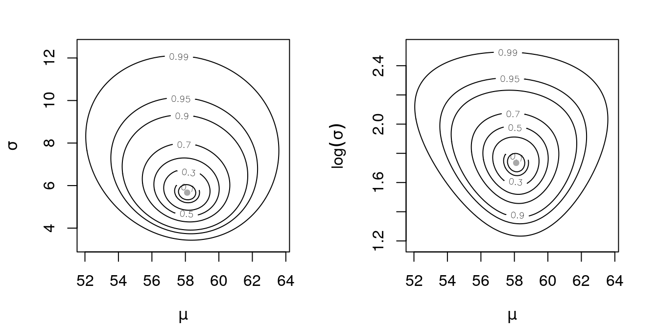
Figure 8: Deviances of (\(\mu, \sigma\)) and (\(\mu, \log \sigma\)) for a Gaussian sample made of interval data.
From Figure 8 two things are important to mention. First, with interval data, the surface doesn’t exhibit orthogonally between the parameters. Second, in the log parametrization of sigma we have better behavior in the surface.
Now, we obtain the likelihood profiles for each parameter. The profiles are presented in Figure 9.
To obtain the likelihood profile for \(\mu\), let’s say, we need to create a grid of values of \(\mu\) and for each value of this grid find the value, let’s say, \(\hat{\sigma}_{\mu}\) that maximizes the profile likelihood. We do this below for \(\mu\) and \(\sigma\), the results can be seen in Figure 9.
# profiles -----------------------------------------------------------------------
# optimizing one parameter per time (optimize routine: single par. optimization)
# we need to split the par argument in two
lkl.norm.profiles <- function(mu, sigma, xs, less.than, more.than) {
    l1 <- sum(dnorm(xs, mean = mu, sd = sigma, log = TRUE))
    l2 <- 5 * log(pnorm(less.than, mean = mu, sd = sigma))
    l3 <- 3 * log(1 - pnorm(more.than, mean = mu, sd = sigma))
    lkl <- l1 + l2 + l3
    return(lkl)}
par(mar = c(4, 4, 2, 2) + .1, mfrow = c(1, 2)) # plot window definition
## mu ----------------------------------------------------------------------------
mu.grid <- seq(45, 69.25, length.out = 100)
# with the optimize routine we obtain two numbers:
# the optimal sigma for the given value of mu.grid, and the log-likelihood value
mu.perf <- matrix(0, nrow = length(mu.grid), ncol = 2)
for (i in 1:length(mu.grid)) {
    mu.perf[i, ] <- unlist(
        optimize(lkl.norm.profiles, lower = 0, upper = 50, mu = mu.grid[i],
                 xs = data, less.than = 65, more.than = 50, maximum = TRUE))}
plot(mu.grid, mu.perf[ , 2], type = "l",
     xlab = expression(mu), ylab = expression(l(mu[sigma])))
abline(v = par.est[1], lty = 2)
## sigma -------------------------------------------------------------------------
sigma.grid <- seq(3.25, 13.75, length.out = 100)
sigma.perf <- matrix(0, nrow = length(sigma.grid), ncol = 2)
for (i in 1:length(sigma.grid)) {
    sigma.perf[i, ] <- unlist(
        optimize(lkl.norm.profiles, lower = 0, upper = 100, sigma = sigma.grid[i],
                 xs = data, less.than = 65, more.than = 50, maximum = TRUE))}
plot(sigma.grid, sigma.perf[ , 2], type = "l",
     xlab = expression(sigma), ylab = expression(l(sigma[mu])))
# we apply the exponential, since we did log sigma optimization by last
abline(v = exp(par.est[2]), lty = 2)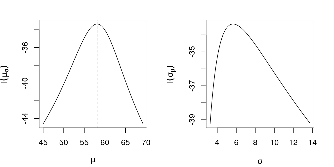
Figure 9: Profile log-likelihoods for \(\mu\) and \(\sigma\) for a Gaussian sample made of interval data. In dashed, the respective MLE’s.
Standard error
Obtain the standard error estimates.
With the \(\texttt{optim}\) routine we obtain the hessian.
init.guess <- c(mean(data), sd(data)) # initial guess
# parameters estimation, now also computing the hessian
(hess <- optim(init.guess, lkl.norm, xs = data,
               less.than = 65, more.than = 50, hessian = TRUE)$hessian)
[,1] [,2]
[1,] 0.38190632 0.04403561
[2,] 0.04403561 0.80092515And we know that the hessian, \(H(\theta)\), is the negative of the observed information, \(I_{O}(\theta)\), and that asymptotically the variance of \(\hat{\theta}\) is \(I_{O}(\theta)^{-1}\). Thus,
(se <- diag(sqrt(1 / hess))) # standard error[1] 1.618160 1.117388The standard errors, se, are
\[ \text{se}(\hat{\mu}) = 1.618, \quad \text{se}(\hat{\sigma}) = 1.117. \]