Poisson regression

Consider a sample of a r.v. $Y$ where it is assumed that $Y_{i} \sim P(\lambda_{i})$ where the parameter $\lambda_{i}$ is described by a function of an explanatory variable $\log (\lambda_{i}) = \beta_{0} + \beta_{1} x_{i}$ with values known from $x_{i}.$ Simulated data with ($\beta_{0} = 2, \beta_{1} = 0.5$) are shown below.

data <- data.frame(y = c(10, 15, 11, 37, 70, 19, 12, 12, 13, 88),
                   x = c(1.7, 1.5, .5, 2.8, 4.4, 1.8, .4, .7, 1.3, 5.1))
par(mar = c(4, 4, 2, 2) + .1)
plot(y ~ x, data)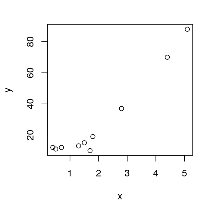

$Dispersion between the variables \texttt{Y} and \texttt{X}.$

Figure 14: Dispersion between the variables and .

Likelihood

Obtain the graph of the likelihood function indicating the position of the true values of the parameters.

The log-likelihood is given by

\[ l(\lambda) = -n \lambda + \log \lambda \sum_{i=1}^{n} y_{i} - \sum_{i=1}^{n} \log y_{i}!~, \quad \lambda_{i} = \exp \{\beta_{0} + \beta_{1} x_{i}\}. \]

# likelihood ---------------------------------------------------------------------
lkl.model.poi <- function(b0, b1, data) {
    n <- nrow(data)
    lambda <- exp(b0 + b1 * data$x)
    lkl <- sum(dpois(data$y, lambda = lambda, log = TRUE))
    # we return the negative of the log-likelihood,
    # since the optim routine performs a minimization
    return(-lkl)
}
# deviance -----------------------------------------------------------------------
dev.model.poi <- function(beta, beta.est, ...) {
    b0 <- beta[1] ; b1 <- beta[2]
    b0.est <- beta.est[1] ; b1.est <- beta.est[2]
    lkl.grid <- lkl.model.poi(b0, b1, ...)
    lkl.est <- lkl.model.poi(b0.est, b1.est, ...)
    lkl.diff <- lkl.grid - lkl.est
    # remember: here we have the negative of the log-likelihoods,
    # so the sign the different
    return(2 * lkl.diff)
}
# deviance, vectorized version ---------------------------------------------------
dev.model.poi.surf <- Vectorize( function(a, b, ...) dev.model.poi(c(a, b), ...) )
# deviance contour, plotting -----------------------------------------------------
b0.grid <- seq(1.625, 2.475, length.out = 100)
b1.grid <- seq(.375, .6, length.out = 100)

outer.grid <- outer(b0.grid, b1.grid, FUN = dev.model.poi.surf,
                    beta.est = c(2, .5), data = data)

contour.levels <- c(.99, .95, .9, .7, .5, .3, .1, .05)
par(mar = c(4, 4, 2, 2) + .1)
contour(b0.grid, b1.grid, outer.grid,
        levels = qchisq(contour.levels, df = 2), labels = contour.levels,
        xlab = expression(beta[0]), ylab = expression(beta[1]))
# true parameter values
points(c(2, .5), pch = 19, cex = .75)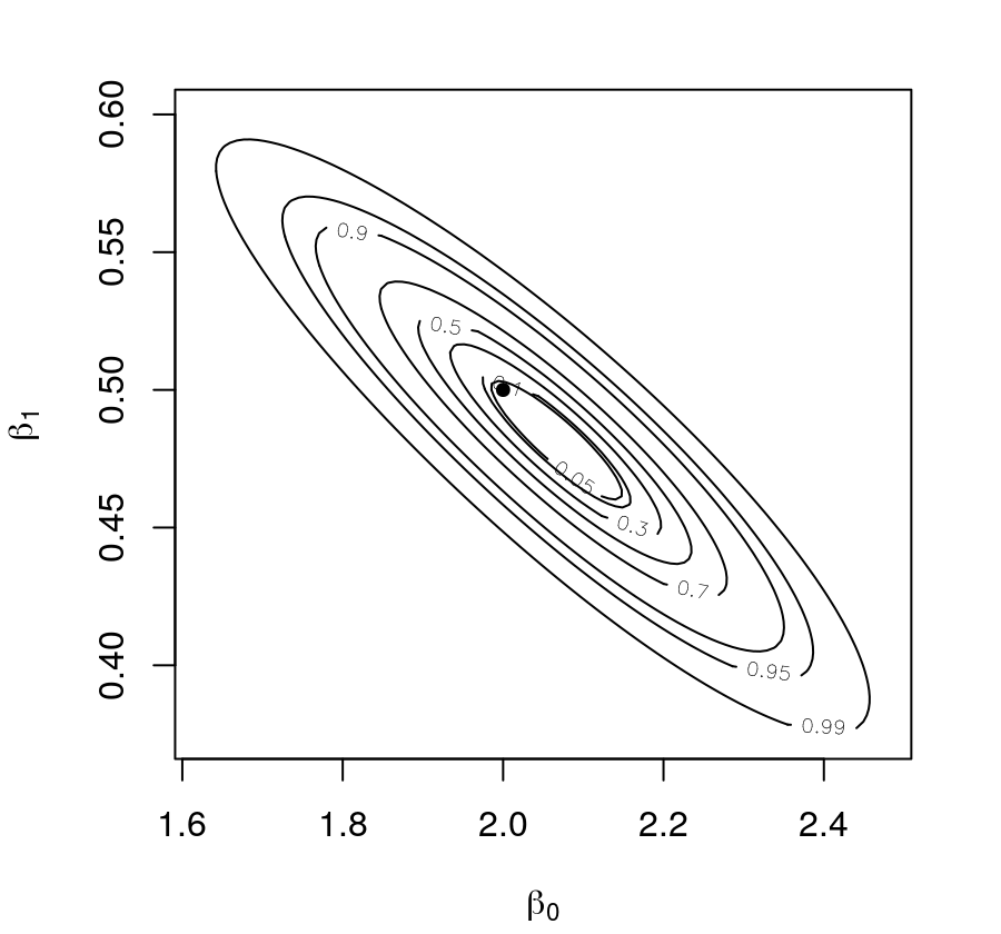

$Deviance of ($\beta_{0}, \beta_{1}$) for a Poisson regression based on \texttt{data}.$

Figure 15: Deviance of ($\beta_{0}, \beta_{1}$) for a Poisson regression based on .

Profile likelihood

Obtain the likelihood profiles of the parameters.

par(mar = c(4, 4, 2, 2) + .1, mfrow = c(1, 2)) # plot window definition
# profiling ----------------------------------------------------------------------
coef.profile <- function(grid, coef = c("b0", "b1")) {
    n <- length(grid) ; prof <- numeric(n)
    for (i in 1:n) {
        # for some points can happen that the hessian not be invertible
        tryCatch({ # with tryCatch we can skip these points
            prof[i] <- switch(
                coef,
                "b0" = mle2(lkl.model.poi, start = list(b1 = .5),
                            data = list(data = data, b0 = grid[i]),
                            method = "BFGS")@details$value,
                "b1" = mle2(lkl.model.poi, start = list(b0 = min(data$y)),
                            data = list(data = data, b1 = grid[i]),
                            method = "BFGS")@details$value)},
            warning = function(w) w)}
    return((-1) * prof)}
# beta_0 -------------------------------------------------------------------------
b0.grid <- seq(1.25, 2.75, length.out = 100)
plot(b0.grid, coef.profile(b0.grid, "b0"), type = "l", xlab = expression(beta[0]),
     ylab = "log-likelihood") ; abline(v = 2, lty = 2)
# beta_1 -------------------------------------------------------------------------
b1.grid <- seq(.3, .675, length.out = 100)
plot(b1.grid, coef.profile(b1.grid, "b1"), type = "l", xlab = expression(beta[1]),
     ylab = "log-likelihood") ; abline(v = .5, lty = 2)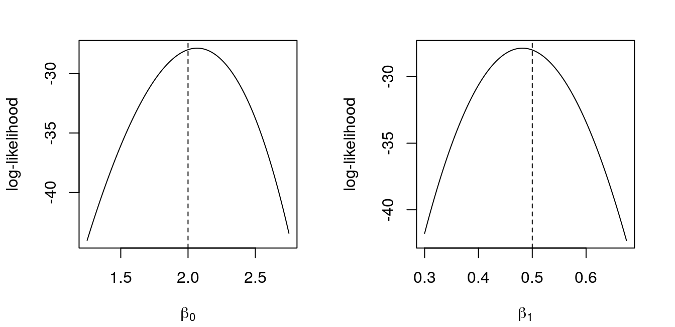

$Profile log-likelihoods for $\beta_{0}$ and $\beta_{1}$ for a Poisson regression. In dashed, MLE's.$

Figure 16: Profile log-likelihoods for $\beta_{0}$ and $\beta_{1}$ for a Poisson regression. In dashed, MLE’s.

MLE

Get estimates.

(par.est <- mle2(lkl.model.poi, start = list(b0 = min(data$y), b1 = 0),
                 data = list(data = data), method = "BFGS"))


Call:
mle2(minuslogl = lkl.model.poi, start = list(b0 = min(data$y), 
    b1 = 0), method = "BFGS", data = list(data = data))

Coefficients:
       b0        b1 
2.0675572 0.4816563 

Log-likelihood: -27.86

Intervals

Get intervals (use different methods).

par(mar = c(4, 4, 2, 2) + .1, mfrow = c(2, 1)) # plot window definition
library(rootSolve) # uniroot.all function
library(numDeriv) # hessian function
# beta_0 -------------------------------------------------------------------------
## first, plotting the profile with point estimates ------------------------------
plot(b0.grid, coef.profile(b0.grid, "b0"), type = "l",
     xlab = expression(beta[0]), ylab = "log-likelihood")
abline(v = 2, lty = 3) ; abline(v = par.est@coef[1], lty = 2)
## intervals ---------------------------------------------------------------------
### probability-based interval ---------------------------------------------------
# cutoff's corresponding to a 95\% confidence interval for beta
# minus, since lkl.model.poi return -lkl
cut <- log(.15) - par.est@details$value ; abline(h = cut, lty = 2)
# finding the cutoff values
ic.poi <- function(grid, coef = c("b0", "b1")) {
    lkl.prof <- switch(
        coef,
        "b0" = mle2(lkl.model.poi, start = list(b1 = 0),
                    data = list(data = data, b0 = grid), method = "BFGS"
        )@details$value,
        "b1" = mle2(lkl.model.poi, start = list(b0 = min(data$y)),
                    data = list(data = data, b1 = grid), method = "BFGS"
        )@details$value)
    (-1) * lkl.prof - cut}
# for some "mysterious" reason the uniroot.all
# doesn't work here, but uniroot works perfectly
ic.95.prob.b0 <- c(uniroot(ic.poi, c(1, par.est@coef[1]), "b0")$root,
                   uniroot(ic.poi, c(par.est@coef[1], 3), "b0")$root)
arrows(x0 = ic.95.prob.b0, y0 = rep(cut, 2),
       x1 = ic.95.prob.b0, y1 = rep(-43.5, 2), lty = 2, length = .1)
### wald confidence interval -----------------------------------------------------
# quadratic approximation
qa.coef.poi <- function(grid, coef = c("b0", "b1")) {
    coef.hat <- switch(coef, "b0" = par.est@coef[1], "b1" = par.est@coef[2])
    lkl.prof <- coef.profile(coef.hat, coef)
    hess <- hessian(coef.profile, x = coef.hat, coef = coef)
    n <- length(grid) ; qa <- numeric(n)
    for (i in 1:n) qa[i] <- lkl.prof + .5 * hess * (grid[i] - coef.hat)**2
    return(qa)}
qa.b0.poi <- qa.coef.poi(b0.grid, "b0") ; lines(b0.grid, qa.b0.poi, col = "darkgray")

cut <- log(.15) + qa.coef.poi(par.est@coef[1], "b0")
abline(h = cut, lty = 2, col = "darkgray")
# now, finding the cutoff values
ic.coef.qa.poi <- function(grid, coef) qa.coef.poi(grid, coef) - cut

wald.95.b0 <- uniroot.all(ic.coef.qa.poi, range(b0.grid), coef = "b0")
arrows(x0 = wald.95.b0, y0 = rep(cut, 2),
       x1 = wald.95.b0, y1 = rep(-43.5, 2), lty = 2, length = .1, col = "darkgray")
### from the mle2 output we get the standard error of each parameter -------------
se.b0 <- summary(par.est)@coef[1, 2]
mle2.95.b0 <- par.est@coef[1] + qnorm(c(.025, .975)) * se.b0

arrows(x0 = mle2.95.b0, y0 = rep(cut, 2),
       x1 = mle2.95.b0, y1 = rep(-43.5, 2), lty = 3, length = .1)
# beta_1 -------------------------------------------------------------------------
plot(b1.grid, coef.profile(b1.grid, "b1"), type = "l",
     xlab = expression(beta[1]), ylab = "log-likelihood")
abline(v = .5, lty = 3) ; abline(v = par.est@coef[2], lty = 2)
## intervals ---------------------------------------------------------------------
### probability-based interval ---------------------------------------------------
abline(h = cut, lty = 2) # remember, the cutoff is the same
# for some "mysterious" reason the uniroot.all
# doesn't work here, but uniroot works perfectly
ic.95.prob.b1 <- c(uniroot(ic.poi, c(.2, par.est@coef[2]), "b1")$root,
                   uniroot(ic.poi, c(par.est@coef[2], .8), "b1")$root)
arrows(x0 = ic.95.prob.b1, y0 = rep(cut, 2),
       x1 = ic.95.prob.b1, y1 = rep(-42, 2), lty = 2, length = .1)
### wald confidence interval -----------------------------------------------------
qa.b1.poi <- qa.coef.poi(b1.grid, "b1") ; lines(b1.grid, qa.b1.poi, col = "darkgray")
cut <- log(.15) + qa.coef.poi(par.est@coef[2], "b1")
abline(h = cut, lty = 2, col = "darkgray")

wald.95.b1 <- uniroot.all(ic.coef.qa.poi, range(b1.grid), coef = "b1")
arrows(x0 = wald.95.b1, y0 = rep(cut, 2),
       x1 = wald.95.b1, y1 = rep(-42, 2), lty = 2, length = .1, col = "darkgray")
### mle2 standard error of -------------------------------------------------------
se.b1 <- summary(par.est)@coef[2, 2]
mle2.95.b1 <- par.est@coef[2] + qnorm(c(.025, .975)) * se.b1

arrows(x0 = mle2.95.b1, y0 = rep(cut, 2),
       x1 = mle2.95.b1, y1 = rep(-42, 2), lty = 3, length = .1)

$Profile log-likelihoods, in black, for $\beta_{0}$ and $\beta_{1}$ in a Poisson regression with some intervals. In black dotted, the original parameter value. In black dashed, the MLE. The gray curve is a quadratic approx. for the profile, with the gray dashed arrows corresponding to its 95\% interval. The black dashed arrows correspond to the 95\% interval based in a cut in the likelihood. The black dotted arrows correspond to the 95\% interval based in the \texttt{mle2} output.$

Figure 17: Profile log-likelihoods, in black, for $\beta_{0}$ and $\beta_{1}$ in a Poisson regression with some intervals. In black dotted, the original parameter value. In black dashed, the MLE. The gray curve is a quadratic approx. for the profile, with the gray dashed arrows corresponding to its 95% interval. The black dashed arrows correspond to the 95% interval based in a cut in the likelihood. The black dotted arrows correspond to the 95% interval based in the output.

By the amount of code provided in this question, we can see that isn’t so straightforward to obtain intervals and quadratic approximations of profiled likelihoods of parameters.

A very nice and interesting thing that we can see in Figure 17 is how all the three obtained intervals match. A brief, but enough, description is already given in the Figure caption, and for more details, you have the provided code.

Did we obtained the right values?

Compare the previous results with those provided by the $\texttt{glm()}$ function and discuss the findings.

# fitting the model via glm() ----------------------------------------------------
model.glm <- glm(y ~ x, data, family = poisson)
# parameter estimates ------------------------------------------------------------
model.glm$coef

(Intercept)           x 
  2.0675451   0.4816599

# at three decimal cases, the estimates are equal
round(model.glm$coef, 3) == round(par.est@coef, 3)

(Intercept)           x 
       TRUE        TRUE

# maximum log-likelihood ---------------------------------------------------------
logLik(model.glm)

'log Lik.' -27.85527 (df=2)

# at eight decimal cases, the max. log-likes are equal
round(logLik(model.glm), 8) == round(par.est@details[[2]] * (-1), 8)

[1] TRUE

# standard erros -----------------------------------------------------------------
summary(model.glm)$coef[ , 2]

(Intercept)           x 
 0.13201821  0.03494989

## at six decimal cases, the standard errors are equal
round(summary(model.glm)$coef[ , 2], 6) == round(summary(par.est)@coef[ , 2], 6)

(Intercept)           x 
       TRUE        TRUE

As a general reference guide for questions 2 to 6, I read and used (in portuguese): MCIE

@conference{mcie,
  author    = {Wagner Hugo Bonat and Paulo Justiniano RIbeiro Jr and
               Elias Teixeira Krainski and Walmes Marques Zeviani},
  title     = {Computational Methods in Statistical Inference},
  year      = {2012},
  publisher = {20th National Symposium on Probability and Statistics (SINAPE)},
  address   = {Jo\~{a}o Pessoa - PB - Brazil},
}