Hypergeometric distribution
In order to obtain an audience estimate of a game without using ticket sales data or stadium roulette records, special shirts were distributed to 300 supporters on condition that they were used during a game. During the game 250 fans were randomly selected and 12 of them had the shirt.
Likelihood
Obtain the likelihood function for the total number of supporters.
We have here a random variable, let’s say, \(X\), representing the number of observed successes, \(k\). Here an observed success is select a fan using a special shirt. So, we have
\[ X \sim \text{Hypergeometric}(N, K = 300, n = 250), \] with probability \(p = K/N\).
\(N\) is the population size, that we want estimate. \(K\) is the unknown number of fans using a special shirt, and \(n\) is the number of, randomly, selected fans.
\[ \begin{align*} \text{Pr}[X = k] &= \frac{\binom{K}{k} \binom{N-K}{n-k}}{\binom{N}{n}}\\ \text{Pr}[X = 12] &= \frac{\binom{300}{12} \binom{N-300}{250-12}}{\binom{N}{250}}\\ &= \frac{300!~250!}{288!~238!~12!} \frac{(N-300)!~(N-250)!}{(N-538)!~N!}\\ &= \text{constant} \times \frac{(N-300)!~(N-250)!}{(N-538)!~N!}. \end{align*} \]
Since we already have a \(k\), the likelihood is equal to \(\text{Pr}[X = k]\).
\[ \begin{align*} L(N) &= \text{Pr}[X = 12] = \text{constant} \frac{(N-300)!~(N-250)!}{(N-538)!~N!}\\ l(N) = \log L(N) &= \log~\text{constant} + \log~\frac{(N-300)!~(N-250)!}{(N-538)!~N!}\\ &\approx \log~\frac{(N-300)!~(N-250)!}{(N-538)!~N!}. \end{align*} \]
A plot of the likelihood is provided in Figure 5.
# likelihood ---------------------------------------------------------------------
lkl.hypergeo <- function(N, n, K, k) {
    l1 <- lgamma(N - K + 1)
    l2 <- lgamma(N - n + 1)
    l3 <- lgamma(N - K - n + k + 1)
    l4 <- lgamma(N + 1)
    lkl <- l1 + l2 - l3 - l4
    return(lkl)
}
compute.lkl <- function(grid, n, K, k) {
    size.grid = length(grid)
    lkl.grid = numeric(size.grid)
    i = 1
    for (j in grid) {
        lkl.grid[i] = lkl.hypergeo(N = j, n = n, K = K, k = k)
        i = i + 1
    }
    return(lkl.grid)
}
# plotting
par(mar = c(4, 4, 2, 2) + .1)
layout(matrix(c(0, 1, 1, 0,
                2, 2, 3, 3), nrow = 2, byrow = TRUE)) # plot window definition

n.grid <- seq(3000, 17000, by = 20)
plot(n.grid, compute.lkl(n.grid, n = 250, K = 300, k = 12),
     type = "l", xlab = "N", ylab = "log-likelihood")
abline(v = 6250, lty = 2)

n.grid <- seq(539, 1e4, by = 20)
plot(n.grid, compute.lkl(n.grid, n = 250, K = 300, k = 12),
     type = "l", xlab = "N", ylab = "log-likelihood")
abline(v = 6250, lty = 2)

n.grid <- seq(5000, 8000, by = 10)
plot(n.grid, compute.lkl(n.grid, n = 250, K = 300, k = 12),
     type = "l", xlab = "N", ylab = "log-likelihood")
abline(v = 6250, lty = 2)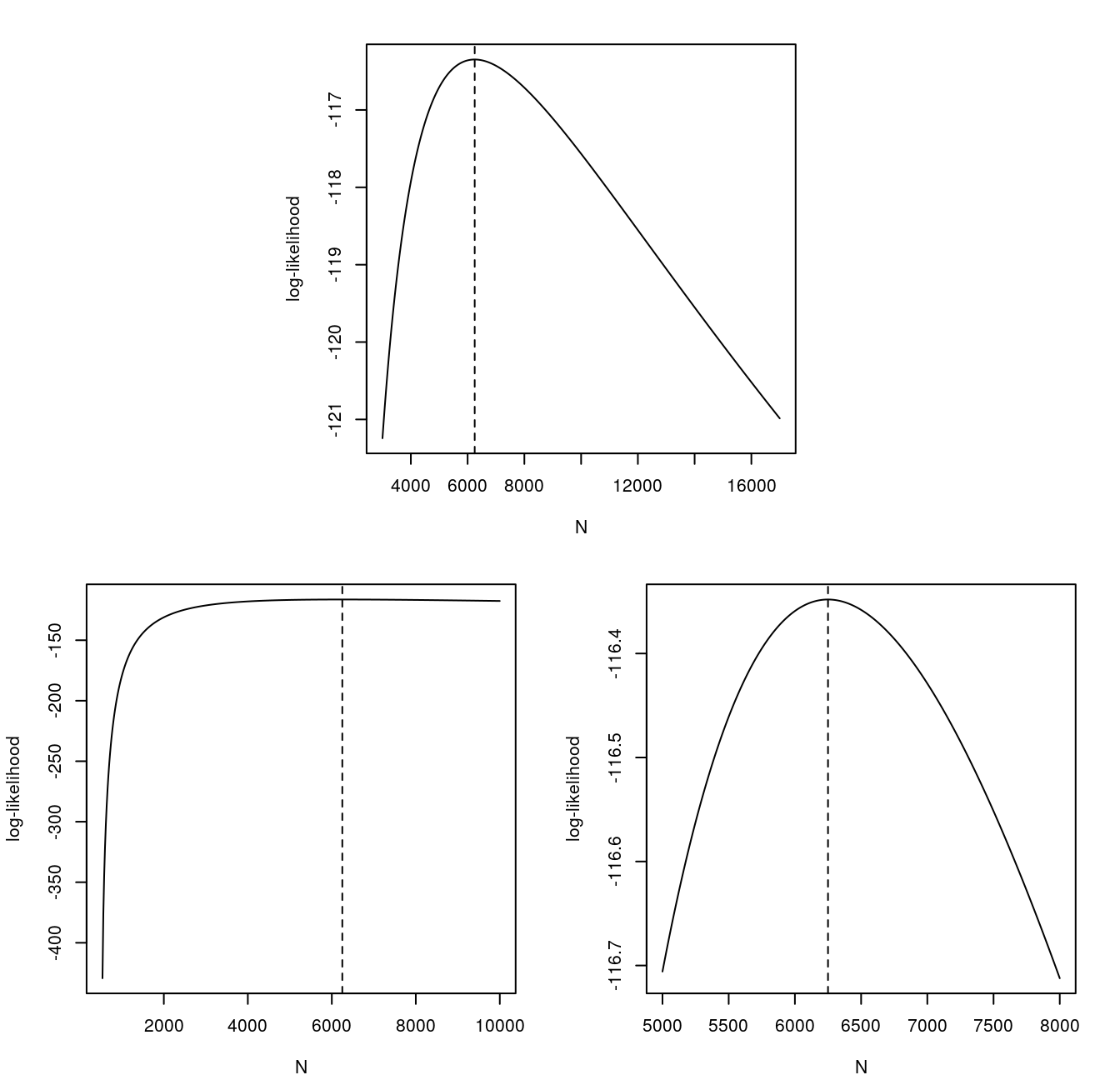
Figure 5: log-likelihood of \(N\) in Hypergeometric(N, K = 300, n = 250) based on \(k = 12\). In dashed, the MLE. Different ranges of \(N\) to have a better understanding of the likelihood behaviour.
The MLE here is given by \(\hat{N} = \left\lfloor Kn/k \right\rfloor = 6250\).
Figure 5 present some very interesting behaviours.
In the top, going from \(N = 3000\) to \(N = 17000\) we can see clearly the likelihood asymmetry. In the bottomleft, starting from the first valid possible value, 539, we see basically nothing. i.e., we don’t see any possible curvature in the likelihood. In the bottomright we focus around the MLE to see better the curvature. Around that point we see a very small variation in the likelihood, \(0.3\), for a range of \(3000\) in \(N\). This shows how smooth is the curvature around the MLE in a large region.
MLE and intervals
Get the point estimate and the interval estimate, the latter by at least two different methods.
# point estimate -----------------------------------------------------------------
optimize(lkl.hypergeo, n = 250, K = 300, k = 12,
         lower = 539, upper = 2e4, maximum = TRUE)
$maximum
[1] 6249.502
$objective
[1] -116.3481Using the routine to do the optimization we obtain \(\hat{N} = 6249.5\), and a log-likelihood of -116.35. This value for \(\hat{N}\) is practically equal to what the ML theory says, \(\hat{N} = \left\lfloor Kn/k \right\rfloor = 6250\).
Next, we compute a quadratic approximation for the hypergeometric (log-)likelihood followed by two intervals, one based in the likelihood, and a wald interval based in the quadratic approximation. All this is presented in Figure 6.
# quadratic approximation of the likelihood --------------------------------------
hess <- numDeriv:::hessian(lkl.hypergeo,
                           x = 6250, n = 250, K = 300, k = 12)
# quadratic approx.
quadprox.hypergeo <- function(N, N.est = 6250, n, K, k) {
    obs.info <- as.vector(-hess) # observed information
    lkl <- lkl.hypergeo(N.est, n, K, k)
    lkl - .5 * obs.info * (N - N.est)**2
}
par(mar = c(4, 4, 2, 2) + .1)
layout(matrix(c(1, 2, 3, 3), nrow = 2, byrow = TRUE),
       heights = c(1.5, 1)) # plot window definition
# likelihood plot
n.grid <- seq(3000, 17000, by = 20)
plot(n.grid, compute.lkl(n.grid, n = 250, K = 300, k = 12),
     type = "l", xlab = "N", ylab = "log-likelihood")
abline(v = 6250, lty = 3)

# quadratic approximation plot
curve(quadprox.hypergeo(x, n = 250, K = 300, k = 12),
      col = "darkgray", add = TRUE)

legend(10500, 318.25, c("log-like", "Quadratic\napprox.", "MLE"),
       col = c(1, "darkgray", 1), lty = c(1, 1, 3), bty = "n")
# intervals for N ----------------------------------------------------------------
# first, we plot again the likelihood and the quadratic approx.
n.grid <- seq(2500, 12000, by = 20)

plot(n.grid, compute.lkl(n.grid, n = 250, K = 300, k = 12),
     type = "l", xlab = "N", ylab = "log-likelihood")
abline(v = 6250, lty = 3)

curve(quadprox.hypergeo(x, n = 250, K = 300, k = 12),
      col = "darkgray", add = TRUE)
## probability-based interval ----------------------------------------------------
# cutoff's corresponding to a 95\% confidence interval for N
cut <- log(.15) + lkl.hypergeo(6250, n = 250, K = 300, k = 12)
abline(h = cut, lty = 2)

ic.lkl.hypergeo <- function(grid, n = 250, K, k) {
    compute.lkl(grid, n, K, k) - cut
}
ic.95.prob <- rootSolve::uniroot.all(ic.lkl.hypergeo, range(n.grid),
                                     K = 300, k = 12)
arrows(x0 = ic.95.prob, y0 = rep(cut, 2),
       x1 = ic.95.prob, y1 = rep(309.5, 2), lty = 2, length = .1)
## wald confidence interval ------------------------------------------------------
cut <- log(.15) + quadprox.hypergeo(6250, n = 250, K = 300, k = 12)
abline(h = cut, lty = 2, col = "darkgray")

se.n.est <- sqrt(as.vector(-1 / hess))
wald.95 <- 6250 + qnorm(c(.025, .975)) * se.n.est

arrows(x0 = wald.95, y0 = rep(cut, 2),
       x1 = wald.95, y1 = rep(309.5, 2), lty = 2, length = .1, col = "darkgray")
# a better look in the approximation around the MLE ------------------------------
n.grid <- seq(5000, 8000, by = 10)

plot(n.grid, compute.lkl(n.grid, n = 250, K = 300, k = 12),
     type = "l", xlab = "N", ylab = "log-likelihood")
abline(v = 6250, lty = 3)
curve(quadprox.hypergeo(x, n = 250, K = 300, k = 12),
      col = "darkgray", add = TRUE)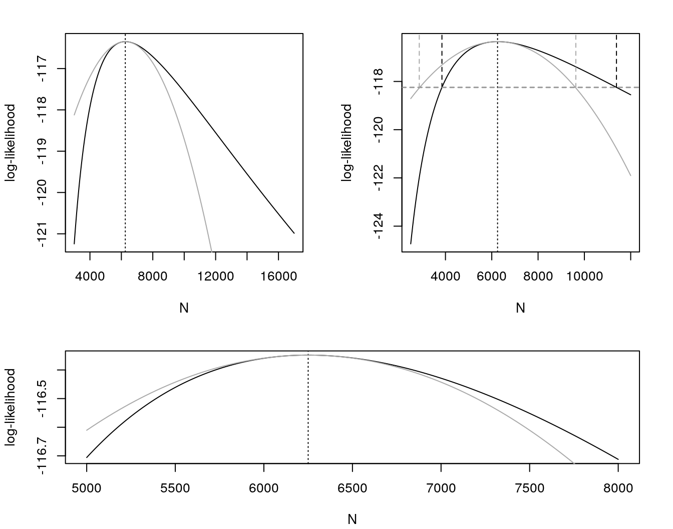
Figure 6: log-likelihood function and MLE of \(N\) in Hypergeometric(N, K = 300, n = 250) based on \(k = 12\). In the topleft, a quadratic approximation in gray. In the topright, two intervals for \(N\) - one based in the likelihood (in black) and one based in the quadratic approximation (in gray). In the bottom we provide a better look in the quadratic approximation.
The quadratic approximation and the intervals were obtained in the same way that in the exercises before, with the only difference that here the hessian was obtained numerically, just for simplicity.
Based in a cut in the likelihood, we obtain \((`r paste(round(ic.95.prob, 0))`)\) as a 95% interval for the total number of fans in the game. With the wald interval (quadratic approximation) we obtain \((2869, 9631)\) as a 95% interval. A considerable difference.
Again but different
Repeat and compare the results if there were 500 shirts and 20 with shirts out of the 250.
The procedure here is exactly the same.
We have
\[ \begin{align*} \text{Pr}[X = k] = \frac{\binom{K}{k} \binom{N-K}{n-k}}{\binom{N}{n}}, \qquad \text{Pr}[X = 20] &= \frac{\binom{500}{20} \binom{N-500}{250-20}}{\binom{N}{250}}\\ &= \frac{500!~250!}{480!~230!~20!} \frac{(N-500)!~(N-250)!}{(N-730)!~N!}\\ &= \text{constant} \times \frac{(N-500)!~(N-250)!}{(N-730)!~N!}. \end{align*} \]
With likelihood
\[ \begin{align*} L(N) &= \text{Pr}[X = 20] = \text{constant} \frac{(N-500)!~(N-250)!}{(N-730)!~N!}\\ l(N) = \log L(N) &= \log~\text{constant} + \log~\frac{(N-500)!~(N-250)!}{(N-730)!~N!}\\ &\approx \log~\frac{(N-500)!~(N-250)!}{(N-730)!~N!}. \end{align*} \]
In Figure 7 we provide the likelihood graphs and intervals for \(N\).
The MLE is exactly the same that the one in the previous scenario, since
\[ \hat{N} = \left\lfloor Kn/k \right\rfloor = \left\lfloor 300 \times 250~/~12 \right\rfloor = \left\lfloor 500 \times 250~/~20 \right\rfloor = 6250. \]
- Based in a cut in the likelihood, we obtain \((`r paste(round(ic.95.prob, 0))`)\) as a 95% interval for the total number of fans in the game. + With the wald interval (quadratic approximation) we obtain \((2869, 9631)\) as a 95% interval for the total number of fans.
A considerable difference.
# plotting -----------------------------------------------------------------------
par(mar = c(4, 4, 2, 2) + .1)
layout(matrix(c(1, 2, 3, 3), nrow = 2, byrow = TRUE),
       heights = c(1.5, 1)) # plot window definition
## likelihood --------------------------------------------------------------------
n.grid <- seq(3000, 17000, by = 20)

plot(n.grid, compute.lkl(n.grid, n = 250, K = 500, k = 20),
     type = "l", xlab = "N", ylab = "log-likelihood")
abline(v = 6250, lty = 3)
## quadratic approximation -------------------------------------------------------
hess <- numDeriv:::hessian(lkl.hypergeo, x = 6250,
                           n = 250, K = 500, k = 20)
curve(quadprox.hypergeo(x, n = 250, K = 500, k = 20),
      col = "darkgray", add = TRUE)
legend(10500, 382.5, c("log-like", "Quadratic\napprox.", "MLE"),
       col = c(1, "darkgray", 1), lty = c(1, 1, 3), bty = "n")
# intervals for N ----------------------------------------------------------------
# first, we plot again the likelihood and the quadratic approx.
n.grid <- seq(2750, 11000, by = 20)

plot(n.grid, compute.lkl(n.grid, n = 250, K = 500, k = 20),
     type = "l", xlab = "N", ylab = "log-likelihood")
abline(v = 6250, lty = 3)

curve(quadprox.hypergeo(N = x, n = 250, K = 500, k = 20),
      col = "darkgray", add = TRUE)
## probability-based interval ----------------------------------------------------
# cutoff's corresponding to a 95\% confidence interval for N
cut <- log(.15) + lkl.hypergeo(6250, n = 250, K = 500, k = 20)
abline(h = cut, lty = 2)

ic.95.prob <- rootSolve::uniroot.all(ic.lkl.hypergeo, range(n.grid),
                                     K = 500, k = 20)
arrows(x0 = ic.95.prob, y0 = rep(cut, 2),
       x1 = ic.95.prob, y1 = rep(370.25, 2), lty = 2, length = .1)
## wald confidence interval ------------------------------------------------------
cut <- log(.15) + quadprox.hypergeo(6250, n = 250, K = 500, k = 20)
abline(h = cut, lty = 2, col = "darkgray")

se.n.est <- sqrt(as.vector(-1 / hess))
wald.95 <- 6250 + qnorm(c(.025, .975)) * se.n.est

arrows(x0 = wald.95, y0 = rep(cut, 2),
       x1 = wald.95, y1 = rep(370.25, 2), lty = 2, length = .1, col = "darkgray")
# a better look in the approximation around the MLE ------------------------------
n.grid <- seq(5000, 7500, by = 10)

plot(n.grid, compute.lkl(n.grid, n = 250, K = 500, k = 20),
     type = "l", xlab = "N", ylab = "log-likelihood")
abline(v = 6250, lty = 3)
curve(quadprox.hypergeo(x, n = 250, K = 500, k = 20),
      col = "darkgray", add = TRUE)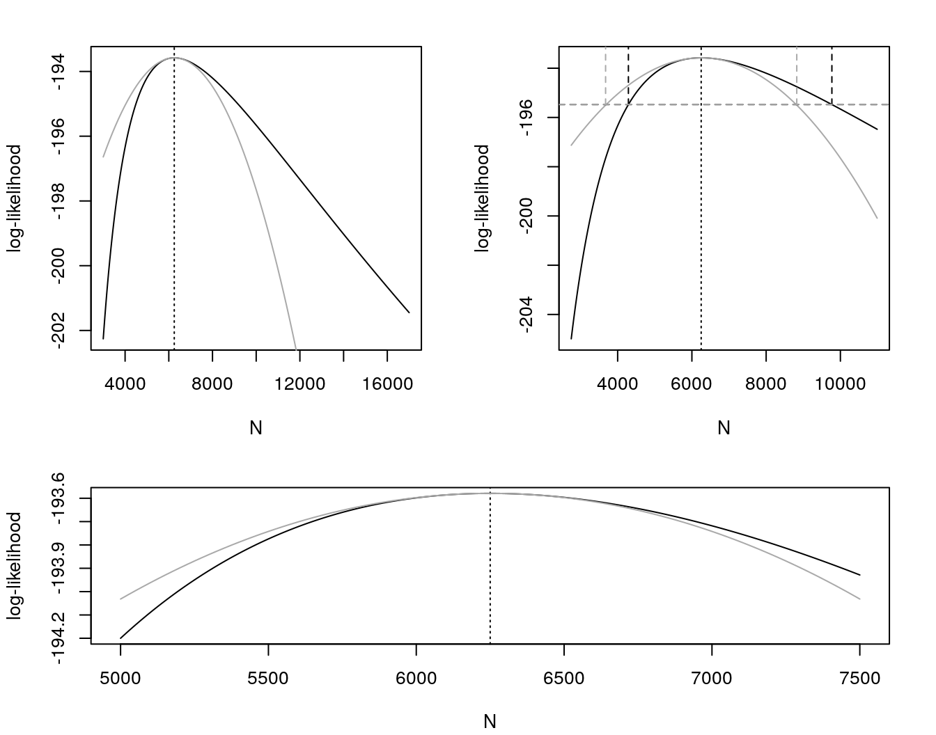
Figure 7: log-likelihood function and MLE of \(N\) in Hypergeometric(N, K = 500, n = 250) based on \(k = 20\). In the topleft, a quadratic approximation in gray. In the topright, two intervals for \(N\) - one based in the likelihood (in black) and one based in the quadratic approximation (in gray). In the bottom we provide a better look in the quadratic approximation.
Comparing with the previous scenario the intervals changed considerably, even with MLE retain the same.
The likelihood shape is the same that before, just with a vertical increase. Before the maximum log-likelihood estimate was around 318, now is around 382.