Poisson regression (extra)
Poisson regression (focus on the profile likelihood)
In the previous exercise, we computed the profile likelihood for each parameter of a simple Poisson regression with just one covariate, i.e., an intercept, \(\beta_{0}\), and an angular coefficient, \(\beta_{1}\).
Together with the profile and an interval based in a cut in this profile likelihood (let’s say, a probability-based interval), we did a quadratic approximation in this profile likelihood. In the “real” world with “real” problems this isn’t a very smart thing to do, but here just as an exercise, I believe that is extremely valid.
Using the same functions created before, we first show, in black, in Figure 18, the profiles likelihood together with its respective quadratic approximations.
Now, something that we can look at is to the estimated likelihood (as \(\texttt{Pawitan}\) calls). In the profiled one, for \(\beta_{0}\) let’s say, in a grid of \(\beta_{0}\)’s, we estimate the \(\beta_{1}\)’s and then get the corresponding likelihoods. In the estimated one, as the name suggests, we fix \(\beta_{1}\) in it’s estimate, and in a grid of \(\beta_{0}\)’s, we get the likelihoods.
The estimated likelihood for each parameter and its correspondent quadratic approximation is computed and presented, in gray, in Figure 18.
# lkl.est.poi: estimated  poisson likelihood -------------------------------------
lkl.est.poi <- function(grid, coef = c("b0", "b1")) {
    coef.hat <- switch(coef, "b0" = par.est@coef[2], "b1" = par.est@coef[1])
    n <- length(grid)
    lkl.est <- numeric(n)
    for (i in 1:n) {
        lkl.est[i] <- switch(
            coef,
            "b0" = lkl.model.poi(b0 = grid[i], b1 = coef.hat, data = data),
            "b1" = lkl.model.poi(b0 = coef.hat, b1 = grid[i], data = data))
    }
    return((-1) * lkl.est)
}
# qa.est.poi: quadratic approximation of the estimated poisson likelihood --------
qa.est.poi <- function(grid, coef = c("b0", "b1")) {
    coef.hat <- switch(coef, "b0" = par.est@coef[1], "b1" = par.est@coef[2])
    lkl.hat <- -par.est@min
    hess <- switch(coef,
                   "b0" = -par.est@details$hessian[1],
                   "b1" = -par.est@details$hessian[4])
    n <- length(grid)
    qa <- numeric(n)
    for (i in 1:n) {
        qa[i] <- switch(coef,
                        "b0" = lkl.hat + .5 * hess * (grid[i] - coef.hat)**2,
                        "b1" = lkl.hat + .5 * hess * (grid[i] - coef.hat)**2)
    }
    return(qa)
}
# --------------------------------------------------------------------------------
par(mar = c(4, 4, 2, 2) + .1, mfrow = c(2, 1)) # plot window definition
# beta_0 -------------------------------------------------------------------------
## first, plotting the profile with point estimate -------------------------------
b0.profile <- coef.profile(b0.grid, "b0")

plot(b0.grid, b0.profile, type = "l",
     xlab = expression(beta[0]), ylab = "log-likelihood")
abline(v = par.est@coef[1], lty = 3)
## now, the quadratic approximation of the profile -------------------------------
lines(b0.grid, qa.b0.poi, lty = 2)
## performing and plotting the conditional likelihood ----------------------------
lkl.est.b0.poi <- lkl.est.poi(b0.grid, "b0")
lines(b0.grid, lkl.est.b0.poi, col = "darkgray")
## performing and plotting the quadratic approx. of the estimated likelihood -----
qa.est.b0.poi <- qa.est.poi(b0.grid, "b0")
lines(b0.grid, qa.est.b0.poi, col = "darkgray", lty = 2)
# beta_1 -------------------------------------------------------------------------
b1.profile <- coef.profile(b1.grid, "b1")

plot(b1.grid, b1.profile, type = "l",
     xlab = expression(beta[1]), ylab = "log-likelihood")
abline(v = par.est@coef[2], lty = 3)

lines(b1.grid, qa.b1.poi, lty = 2)

lkl.est.b1.poi <- lkl.est.poi(b1.grid, "b1")
lines(b1.grid, lkl.est.b1.poi, col = "darkgray")

qa.est.b1.poi <- qa.est.poi(b1.grid, "b1")
lines(b1.grid, qa.est.b1.poi, col = "darkgray", lty = 2)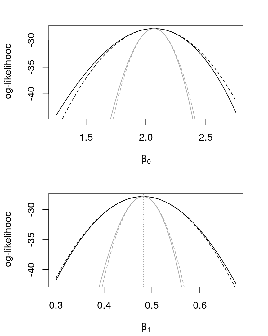
Figure 18: Profile log-likelihoods and quadratic approximations, in black (solid and dashed, respectively), for \(\beta_{0}\) and \(\beta_{1}\) in a Poisson regression. In dotted, the MLE. Estimated log-likelihoods and quadratic approximations, in gray (solid and dashed, respectively).
The first and important note that we can take from Figure 18, and that makes all the possible sense, is how the estimated likelihood is narrow (compared with the profiled one). The explanation for this is that in the estimated situation it’s assumed as known one of the coefficients, fixing it at the MLE. In the other hand, the profile likelihood takes into account that one of the coefficients is unknown. Hence, it’s sensible that the profile is greater than the estimated.
Another important point to mention is about the manner that we compute the profile likelihood. A function with this goal was made in the previous question, \(\texttt{qa.coef.poi}\). The important thing to note about these function is that the hessian there is computed from the profile likelihood. This is inefficient, and not necessary. Instead, we can just take the corresponding element in the variance-covariance matrix, invert, and use it. In other words, we don’t need to use the profile likelihood to compute a quadratic approximation to the profile likelihood. We implement this in \(\texttt{smart.qa.coef.poi}\).
# qa: quadratic approximation ----------------------------------------------------
smart.qa.coef.poi <- function(model.mle2, coef = c("b0", "b1"), grid) {
    coef.hat <- switch(coef, "b0" = model.mle2@coef[1], "b1" = model.mle2@coef[2])
    lkl.hat <- (-1) * model.mle2@details$value
    hess <- switch(coef,
                   "b0" = (-1) / model.mle2@vcov[1],
                   "b1" = (-1) / model.mle2@vcov[4])
    n <- length(grid) ; qa <- numeric(n)
    for (i in 1:n) {
        qa[i] <- switch(coef,
                        "b0" = lkl.hat + .5 * hess * (grid[i] - coef.hat)**2,
                        "b1" = lkl.hat + .5 * hess * (grid[i] - coef.hat)**2)}
    return(qa)}
# --------------------------------------------------------------------------------
par(mar = c(4, 4, 2, 2) + .1)
layout(matrix(1:4, 2, 2), widths = c(1.5, 1)) # plot window definition
# beta_0 -------------------------------------------------------------------------
## first, plotting the profile with the point estimate ---------------------------
plot(b0.grid, b0.profile, type = "l", xlab = expression(beta[0]),
     ylab = "log-likelihood") ; abline(v = par.est@coef[1], lty = 3)
## now, the "old" quadratic approximation of the profile -------------------------
lines(b0.grid, qa.b0.poi, lty = 2)
## and finally, the new and smart quadratic approximation of the profile ---------
sqa.b0.poi <- smart.qa.coef.poi(model.mle2 = par.est, coef = "b0", grid = b0.grid)
lines(b0.grid, sqa.b0.poi, col = "gray")
# beta_1 -------------------------------------------------------------------------
plot(b1.grid, b1.profile, type = "l", xlab = expression(beta[1]),
     ylab = "log-likelihood") ; abline(v = par.est@coef[2], lty = 3)
lines(b1.grid, qa.b1.poi, lty = 2)

sqa.b1.poi <- smart.qa.coef.poi(model.mle2 = par.est, coef = "b1", grid = b1.grid)
lines(b1.grid, sqa.b1.poi, col = "gray")
# how much the quadratic approximations are similar? -----------------------------
compare.qas <- function(dp, coef = c("b0", "b1")) {
    compare <- numeric(dp)
    for (i in 1:dp) {
        compare[i] <- switch(
            coef,
            "b0" = table(round(sqa.b0.poi, i) == round(qa.b0.poi, i))["TRUE"],
            "b1" = table(round(sqa.b1.poi, i) == round(qa.b1.poi, i))["TRUE"])}
    compare[is.na(compare)] <- 0
    graph <- plot(compare, type = "h",
                  xlab = "decimal places", ylab = "% of matching")
    return(invisible(graph))}
compare.qas(6, "b0") ; compare.qas(6, "b1")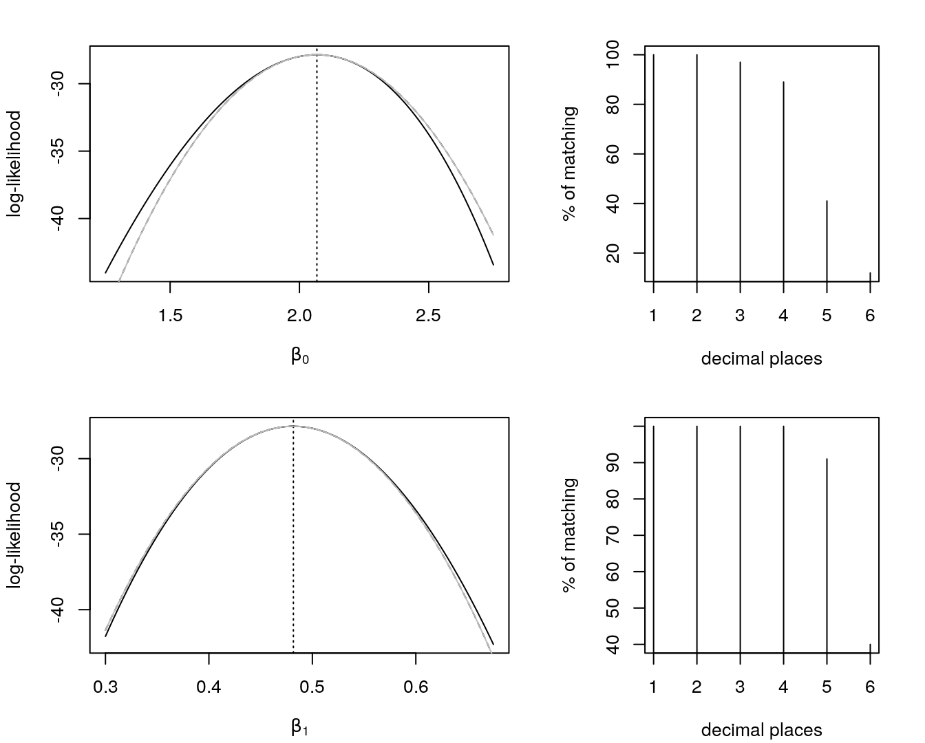
Figure 19: Profile log-likelihoods, solid line, for \(\beta_{0}\) and \(\beta_{1}\) in a Poisson regression. In dotted, MLEs. Quadratic approx.’s of the profiles in black dashed and gray, with a matching percentage between them considering six different decimal places.
In Figure 19 we see that the dashed matches with the gray line, i.e., the quadratic approximations are equal. To see better how equal they’re, the right graphs of Figure 19 show the percentage of matching values (quadratic approximations of the profile log-likelihoods) considering different levels of rounding. As a conclusion statement, they’re quite equal. This completes and complement the last paragraph.
A third and last note is that to compute the quadratic approx. for the estimated likelihood we use the corresponding element of the information matrix. To compute the quadratic approx. for the profile likelihood we use the inverse of that element in the variance-covariance matrix, that is the inverse of the information matrix.
The insights for this exercise was taken from \(\texttt{Pawitan}\)’s book.