Gaussian regression
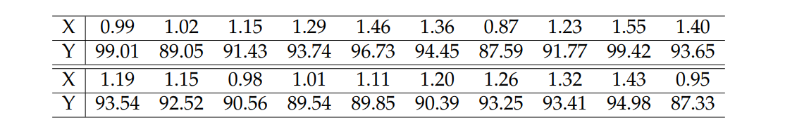
Consider the following data table (adapted/modified from Montgomery & Runger, 1994) to which we wish to fit a simple linear regression model by relating the response variable \(Y\) (purity in %) to an explanatory variable \(X\) (hydrocarbon level).
Likelihood
Find the likelihood function.
data <- data.frame(
    x = c(.99, 1.02, 1.15, 1.29, 1.46, 1.36, .87, 1.23, 1.55, 1.4,
          1.19, 1.15, .98, 1.01, 1.11, 1.2, 1.26, 1.32, 1.43, .95),
    y = c(99.01, 89.05, 91.43, 93.74, 96.73, 94.45, 87.59, 91.77, 99.42,
          93.65, 93.54, 92.52, 90.56, 89.54, 89.85, 90.39, 93.25, 93.41,
          94.98, 87.33))
par(mar = c(4, 4, 2, 2) + .1)
plot(y ~ x, data, xlab = "hydrocarbon level", ylab = expression("purity"~("%")))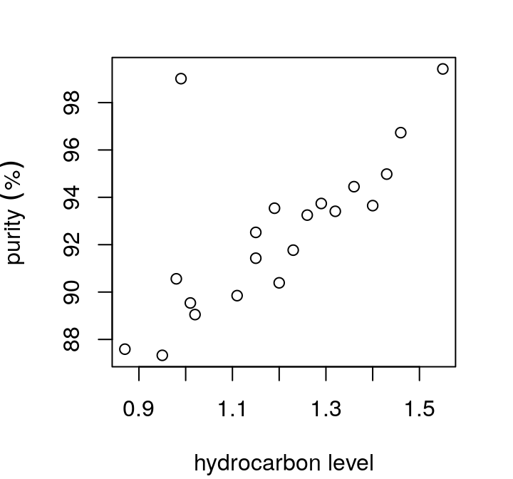
Figure 10: Dispersion between hydrocarbon level \(\times\) purity (%).
Assuming a Normal distribution for \(Y | X\), we have the following log-likelihood, in matricial form
\[ \begin{align*} l(\theta; Y) &= - \frac{n}{2} \log 2\pi - n \log \sigma - \frac{1}{2\sigma^{2}} \left \| Y - X \beta \right \|^{2}\\ &= \text{constant} - n \log \sigma - \frac{1}{2\sigma^{2}} \left \| Y - X \beta \right \|^{2}, \end{align*} \]
were \(\theta = [\beta_{0}~\beta_{1}~\sigma]^{\top}\), \(\beta = [\beta_{0}~\beta_{1}]^{\top}\), and \(\mu_{i} = \beta_{0} + \beta_{1} x_{i}\).
MLE
Find the estimates of maximum likelihood.
# likelihood ---------------------------------------------------------------------
lkl.model.norm <- function(b0, b1, sigma, y, x, logsigma = FALSE) {
    ## if logsigma = TRUE, we do the parametrization using log(sigma)
    if (logsigma) sigma <- exp(sigma)
    mu <- b0 + b1 * x
    lkl <- sum(dnorm(y, mean = mu, sd = sigma, log = TRUE))
    # we return the negative of the log-likelihood,
    # since the optim routine performs a minimization
    return(-lkl)
}
library(bbmle)
par.est <- mle2(lkl.model.norm,
                start = list(b0 = min(data$y), b1 = 1.5, sigma = sd(data$y)),
                data = list(y = data$y, x = data$x), method = "BFGS")
par.est@coef
b0 b1 sigma
77.988429 12.225489 2.343799 Just checking…
lm(y ~ x, data)$coef # beta_0 and beta_1(Intercept) x
77.98996 12.22453 par.est@coef[[3]]**2 # sigma^2[1] 5.493392(summary(lm(y ~ x, data))$sigma**2) * (nrow(data) - 2) / nrow(data)[1] 5.493386Checked, \(\checkmark\).
Joint likelihood
Obtain the joint likelihood for the parameters \(\beta_{0}\) and \(\beta_{1}\):
With \(\sigma\) fixed in its MLE
considering \(\sigma\) fixed with value equal to its estimate.
# deviance -----------------------------------------------------------------------
dev.model.norm <- function(beta, theta.est, ...) {
    b0 <- beta[1] ; b1 <- beta[2]
    b0.est <- theta.est[[1]] ; b1.est <- theta.est[[2]]
    sigma.est <- theta.est[[3]]
    lkl.grid <- lkl.model.norm(b0, b1, sigma.est, ...)
    lkl.est <- lkl.model.norm(b0.est, b1.est, sigma.est, ...)
    lkl.diff <- lkl.grid - lkl.est
    # remember: here we have the negative of the log-likelihoods,
    # so the sign is different
    return(2 * lkl.diff)
}
# deviance, vectorized version ---------------------------------------------------
dev.model.norm.surf <- Vectorize(function(a, b, ...) dev.model.norm(c(a, b), ...))
# deviance contour, plotting -----------------------------------------------------
b0.grid <- seq(67.5, 88.5, length.out = 100)
b1.grid <- seq(3.5, 21, length.out = 100)

outer.grid <- outer(b0.grid, b1.grid, FUN = dev.model.norm.surf,
                    theta.est = par.est@coef, y = data$y, x = data$x)

par(mar = c(4, 4, 2, 2) + .1)
contour.levels <- c(.99, .95, .9, .7, .5, .3, .1, .05)
contour(b0.grid, b1.grid, outer.grid,
        levels = qchisq(contour.levels, df = 2), labels = contour.levels,
        xlab = expression(beta[0]), ylab = expression(beta[1]))
# converting par.est@coef to a matricial object
points(t(par.est@coef[1:2]), col = 1, pch = 19, cex = .75)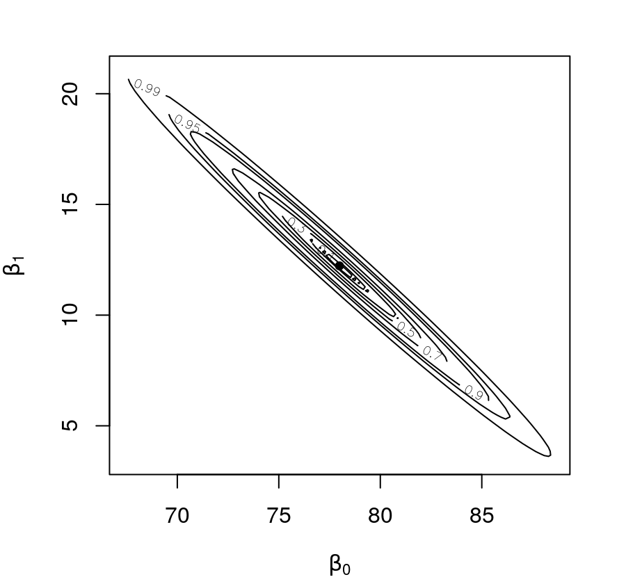
Figure 11: Deviance of (\(\beta_{0}, \beta_{1}\)) with \(\sigma\) fixed in it’s estimative, for a Gaussian regression.
Profile likelihood wrt \(\sigma\)
obtaining the profile likelihood (joint - 2D) with respect to \(\sigma\).
# profile ------------------------------------------------------------------------
sigma.grid <- seq(1.7, 3.5, length.out = 100)
# with the optim routine we obtain three numbers:
# the estimates of beta_0, beta_1, and the log-likelihood value
beta.perf <- matrix(0, nrow = length(sigma.grid), ncol = 3)
for (i in 1:length(sigma.grid)) {
    beta.perf[i, ] <- unlist(
        mle2(lkl.model.norm, start = list(b0 = min(data$y), b1 = 1.5),
             data = list(y = data$y, x = data$x, sigma = sigma.grid[i]),
             method = "BFGS"
        )@details[1:2])
}
par(mar = c(4, 4, 2, 2) + .1)
plot(sigma.grid, -1 * beta.perf[ , 3], type = "l",
     xlab = expression(sigma), ylab = "log-likelihood")
abline(v = par.est@coef[[3]], lty = 2)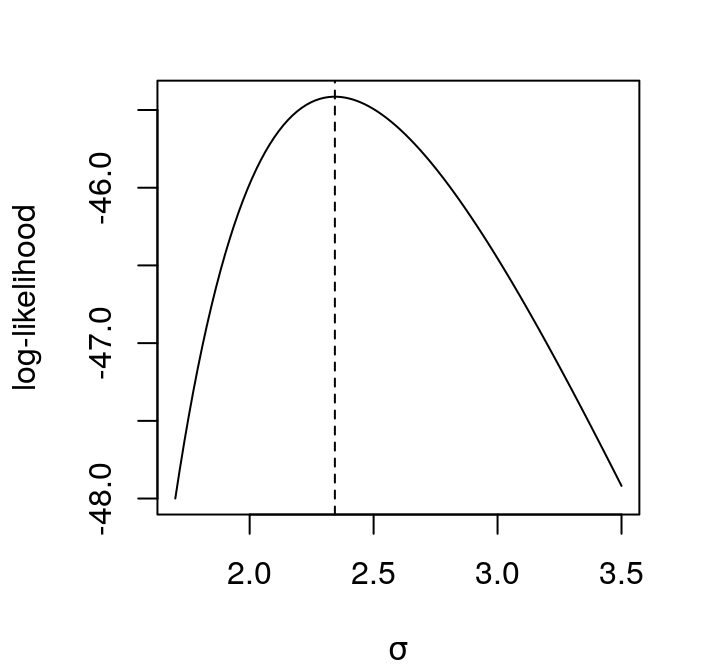
Figure 12: Profile log-likelihood for \(\sigma\), for a Gaussian regression. In dashed, the MLE.
And how the \(\beta\)’s fluctuates across the grid of \(\sigma\)?
summary(beta.perf[ , 1]) # beta_0 Min. 1st Qu. Median Mean 3rd Qu. Max.
77.98 77.99 77.99 77.99 78.00 78.01 summary(beta.perf[ , 2]) # beta_1 Min. 1st Qu. Median Mean 3rd Qu. Max.
12.21 12.22 12.22 12.22 12.22 12.23 Very few, as expected. Since the estimation of \(\beta\) doesn’t depend on \(\sigma\).
Profile likelihood
Obtain the profile likelihood for the parameters \(\beta_{0}\) and \(\beta_{1}\) individually.
par(mfrow = c(1, 2)) # plot window definition, one row and two columns
# profiling ----------------------------------------------------------------------
coef.profile <- function(grid, coef = c("b0", "b1")) {
    n <- length(grid)
    prof <- numeric(n)
    for (i in 1:n) {
        prof[i] <- switch(
            coef,
            "b0" = mle2(lkl.model.norm, start = list(b1 = 1.5),
                        data = list(y = data$y, x = data$x, b0 = grid[i],
                                    sigma = par.est@coef[[3]]),
                        method = "BFGS"
            )@details$value,
            "b1" = mle2(lkl.model.norm, start = list(b0 = min(data$y)),
                        data = list(y = data$y, x = data$x, b1 = grid[i],
                                    sigma = par.est@coef[[3]]),
                        method = "BFGS"
            )@details$value)
    }
    return((-1) * prof)
}
par(mar = c(4, 4, 2, 2) + .1)
# beta_0 -------------------------------------------------------------------------
b0.grid <- seq(67.5, 88.5, length.out = 100)

plot(b0.grid, coef.profile(b0.grid, "b0"), type = "l",
     xlab = expression(beta[0]), ylab = "log-likelihood")

abline(v = par.est@coef[[1]], lty = 2)
# beta_1 -------------------------------------------------------------------------
b1.grid <- seq(3.5, 21, length.out = 100)

plot(b1.grid, coef.profile(b1.grid, "b1"), type = "l",
     xlab = expression(beta[1]), ylab = "log-likelihood")

abline(v = par.est@coef[[2]], lty = 2)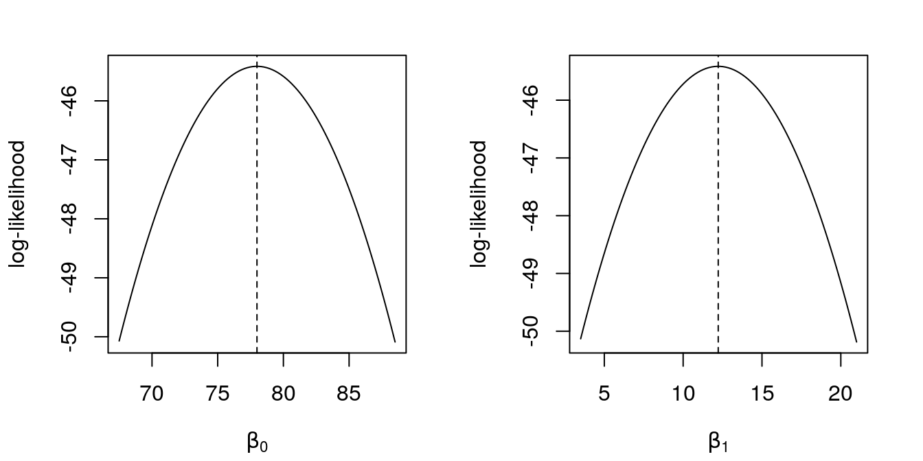
Figure 13: Profile log-likelihoods for \(\beta_{0}\) and \(\beta_{1}\) for a Gaussian regression. In dashed, MLE’s.