Uniform distribution
Let \(X\) be a r.v. with uniform distribution \(X \sim U(0, \theta)\). A random sample gave the following values: 5.5; 3.2; 4, 8, 5.3; 3.8 and 5.0. Obtain the likelihood function and one or more appropriate interval(s) specifying the form of obtaining.
data <- c(5.5, 3.2, 4.8, 5.3, 3.8, 5)The likelihood of a \({\rm Uniform}(0, \theta)\) is
\[\begin{align*} L(\theta) &= \theta^{-n}, \quad \text{for } x_{i} < \theta \text{ for all } i\\ &= \theta^{-n}, \quad \text{for } \theta > x_{(n)}, \end{align*}\] and equal to zero otherwise.
Given the data above, we get \(x_{(n)} = 5.5\) and the likelihood is shown in Figure 1, together with some intervals.
lkl.unif <- function(theta, data) {
    n <- length(data) ; xn <- max(data)
    # this next step, in the way presented, isn't very efficient, since I'll
    # compute the likelihood for all theta's and then, if necessary, convert to
    # zero. however, since we have here a very simple likelihood (and this
    # notation is extremely clear, btw), I keep in this way
    lkl = theta**(-n)*{theta >= xn}
    return(lkl)
}
theta.seq <- seq(4, 12, length.out = 100)
lklseq.unif <- lkl.unif(theta.seq, data)

par(mfrow = c(1, 2), par(mar = c(4, 4, 2, 2) + .1)) # plot window definition
# plotting the normalized likelihood function to have unit maximum
plot(theta.seq, lklseq.unif/max(lklseq.unif), type = "l",
     xlab = expression(theta), ylab = "Likelihood")
# probability-based interval -----------------------------------------------------
# cutoff's corresponding to a 95\% and 99\% confidence interval for the mean
cuts <- c(.15, .04) * lkl.unif(max(data), data) / max(lklseq.unif)
abline(h = cuts, lty = 2:3)
# uniroot.all finds the zeros, so we need to subtract the cutoff point from
# the likelihood to be able to find the points where the likelihood is cut
ic.lkl.unif <- function(theta, cut, ...) {
    lkl.unif(theta, ...)/max(lklseq.unif) - cut
}
ic.95.prob <- rootSolve::uniroot.all(ic.lkl.unif, range(theta.seq),
                                     data = data, cut = cuts[1])
ic.99.prob <- rootSolve::uniroot.all(ic.lkl.unif, range(theta.seq),
                                     data = data, cut = cuts[2])
abline(v = ic.95.prob, lty = 2) ; abline(v = ic.99.prob, lty = 3)

plot(theta.seq, lklseq.unif/max(lklseq.unif), type = "l",
     xlab = expression(theta), ylab = "Likelihood")
# pure likelihood interval -------------------------------------------------------
# cutoff's corresponding to a 95\% and 99\% confidence interval for the mean
cuts <- c(.05, .01) * lkl.unif(max(data), data) / max(lklseq.unif)
abline(h = cuts, lty = 2:3)

ic.95.pure <- rootSolve::uniroot.all(ic.lkl.unif, range(theta.seq),
                                     data = data, cut = cuts[1])
ic.99.pure <- rootSolve::uniroot.all(ic.lkl.unif, range(theta.seq),
                                     data = data, cut = cuts[2])
abline(v = ic.95.pure, lty = 2) ; abline(v = ic.99.pure, lty = 3)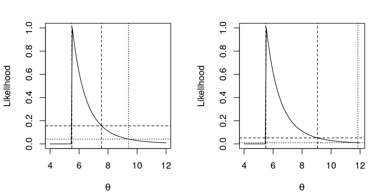
Figure 1: Likelihood function of \(\theta\) in Uniform(0, \(\theta\)) based on \(x_{(6)}\) = 5.5. In the left, likelihood intervals at 15% (dashed line) and 4% (dotted line) cutoff. In the right, likelihood intervals at 5% (dashed line) and 1% (dotted line) cutoff. These cutoffs correspond, in both sides, to a 95% and 99% confidence interval, respectively.
In both graphs of Figure 1 we have two confidence intervals for \(\theta\), one corresponding to a 95% confidence interval (dashed line) and one corresponding to a 99% confidence interval for the mean (dotted line). In the left we have a probability-based likelihood interval, in the right we have a pure likelihood interval.
The left ones are bad intervals, since they’re based in a large-sample theory that results in an exact interval for the Gaussian case, in a good approximation for a reasonably regular case, and as we can see by the figure… here we doesn’t have a regular likelihood (the likelihood isn’t well approximated by a quadratic function), thus, here this interval should not be so good.
Explaining better how we arrived in these intervals:
For a normalized likelihood, \(L(\theta)/L(\hat{\theta})\), we have the following Wilk’s likelihood ratio statistic, defined as \(W\)
\[ W \equiv 2 \log \frac{L(\hat{\theta})}{L(\theta)} \sim \chi_{1}^{2}. \] Its \(\chi^{2}\) distribution is exact only in the normal mean model, and approximately true when the likelihood is reasonably regular.
Based in this Wilk’s statistic we are able to find the probability that the likelihood interval covers \(\theta\),
\[ {\rm Pr}\left\{\frac{L(\theta)}{L(\hat{\theta})} > c\right\} = {\rm Pr}\left\{2 \log \frac{L(\theta)}{L(\hat{\theta})} < -2 \log c \right\} = {\rm Pr}\{\chi_{1}^{2} < -2 \log c\}. \]
So, if for some \(0 < \alpha < 1\) we choose a cutoff
\[ c = e^{-\frac{1}{2} \chi_{1, (1-\alpha)}^{2}}, \]
where \(\chi_{1, (1-\alpha)}^{2}\) is the \(100 (1-\alpha)\) percentile of \(\chi_{1}^{2}\).\
For \(\alpha = 0.05\) and \(0.01\) we have a cutoff \(c = 0.15\) and \(0.04\), that corresponds to a 95% and 99% confidence interval, respectively.
Having the cutoff values we need now to find the interval values, i.e., in which points the cutoff horizontal line cuts the likelihood. For this purpose we use the function \(\texttt{rootSolve::uniroot.all}\).
A likelihood interval at 15% and 4% cutoff for \(\theta\) are (5.5, 7.545) and (5.5, 9.405).
Already on the right side of Figure 1 we have a more coherent, let’s say, confidence interval for the Uniform likelihood. While the likelihood isn’t regular, it is still possible to provide an exact theoretical justification for a confidence interval interpretation. Now
\[ {\rm Pr}\left\{\frac{L(\theta)}{L(\hat{\theta})} > c\right\} = {\rm Pr}\left\{\frac{X_{(n)}}{\theta} > c^{1/n}\right\} = 1 - {\rm Pr}\left\{\frac{X_{(n)}}{\theta} < c^{1/n}\right\} = 1 - (c^{1/n})^{n} = 1 - c. \]
So the likelihood interval with cutoff \(c\) is a \(100 (1-c)\)% confidence interval.
A likelihood interval at 15% and 4% cutoff for \(\theta\) are (5.5, 9.062) and (5.5, 11.849).
Comparing the obtained intervals we see a broader range with the pure likelihood intervals. In other words, with the pure likelihood intervals we see a higher uncertainty than with the (not so recommended here) probability-based likelihood intervals.
For doing this exercise I read and used it Pawitan’s book:
@book{pawitan,
  author    = {Yudi Pawitan},
  title     = {In All Likelihood:
               Statistical Modelling and Inference Using Likelihood},
  year      = {1991},
  publisher = {Oxford University Press},
  address   = {Great Clarendon Street, Oxford OX2 6DP},
}