Poisson distribution
Let \(X\) be a r.v. of a Poisson distribution (\(X \sim P(\lambda)\)) for which the following random sample was obtained: (3, 1, 0, 2, 1, 1, 0, 0).
data <- c(3, 1, 0, 2, 1, 1, 0, 0)Lkl, quad. approx. and intervals
Obtain the likelihood function, its quadratic approximation and intervals for \(\lambda\).
The likelihood and the log-likelihood of a Poisson(\(\lambda\)) is
\[ L(\lambda) = \prod_{i=1}^{n} \frac{e^{-\lambda} \lambda^{x_{i}}}{x_{i}!} \quad \text{and} \quad \log L(\lambda) = l(\lambda) = -n \lambda + \log \lambda \sum_{i=1}^{n} x_{i} - \sum_{i=1}^{n} \log x_{i}!. \]
We work here with the log-likelihood to make our life easier, since the computations are much simpler in the log scale.
By computing the Score (derivative of \(l(\lambda)\) wrt to \(\lambda\)) and making it equal to zero, we find the MLE \(\hat{\lambda} = \bar{x}\). Computing the second derivative we find the observed information
\[ I_{O}(\lambda) = \frac{n \bar{x}}{\lambda^{2}} \quad \rightarrow \quad I_{O}(\hat{\lambda}) = \frac{n}{\bar{x}}. \]
A graph of the Poisson log-likelihood is provided in black in Figure 2.
Doing a quadratic approximation (Taylor expansion of second order) in \(l(\lambda)\) around \(\hat{\lambda}\) we have
\[ \begin{align*} l(\lambda) &\approx l(\hat{\lambda}) + (\lambda - \hat{\lambda}) {l}'(\hat{\lambda}) + \frac{1}{2} (\lambda - \hat{\lambda})^{2} {l}''(\hat{\lambda})\\ &\quad(\text{the Score is zero at the MLE})\\ &= l(\hat{\lambda}) + \frac{1}{2} (\lambda - \hat{\lambda})^{2} {l}''(\hat{\lambda}) = l(\hat{\lambda}) + \frac{1}{2} (\lambda - \hat{\lambda})^{2} I_{O}(\hat{\lambda}). \end{align*} \]
A graph of the quadratic approximation of the Poisson log-likelihood is provided in gray in Figure 2. There we can see how good is the approximation around the maximum likelihood estimator (MLE). Here the sample size is very small, the idea is that as the sample size increase the quality, in this case the range, of the approximation also increase. This should happen because as the sample size increase the Poisson likelihood should be more symmetric.
In the topright graph of Figure 2 we have two intervals for \(\lambda\).
# likelihood ---------------------------------------------------------------------
lkl.poi <- function(lambda, data) {
    n <- length(data)
    # log-likelihood ignoring irrelevant constant terms
    lkl = -n * lambda + sum(data) * log(lambda)
    return(lkl)
}
lambda.seq <- seq(0, 4.5, length.out = 100)
lklseq.poi <- lkl.poi(lambda.seq, data)

par(mar = c(4, 4, 2, 2) + .1)
layout(matrix(c(1, 3, 2, 3), 2, 2), heights = c(1.5, 1)) # plot window definition
plot(lambda.seq, lklseq.poi, type = "l",
     xlab = expression(lambda), ylab = "log-likelihood")
lambda.est <- mean(data) # MLE
abline(v = lambda.est, lty = 3)
# quadratic approximation --------------------------------------------------------
quadprox.poi <- function(lambda, lambda.est, data) {
    n <- length(data)
    obs.info <- n / lambda.est # observed information
    lkl.poi(lambda.est, data) - .5 * obs.info * (lambda - lambda.est)**2
}
curve(quadprox.poi(x, lambda.est, data), col = "darkgray", add = TRUE)
legend(2.4, -6.25, c("log-like", "Quadratic\napprox.", "MLE"),
       col = c(1, "darkgray", 1), lty = c(1, 1, 3), bty = "n")
# intervals for lambda -----------------------------------------------------------
plot(lambda.seq, lklseq.poi, type = "l",
     xlab = expression(lambda), ylab = "log-likelihood")
curve(quadprox.poi(x, lambda.est, data), col = "darkgray", add = TRUE)
abline(v = lambda.est, lty = 3)
## probability-based interval ----------------------------------------------------
# cutoff's corresponding to a 95\% confidence interval for the mean
cut <- log(.15) + lkl.poi(lambda.est, data) ; abline(h = cut, lty = 2)
ic.lkl.poi <- function(lambda, cut, ...) { lkl.poi(lambda, ...) - cut }
ic.95.prob <- rootSolve::uniroot.all(ic.lkl.poi, range(lambda.seq),
                                     data = data, cut = cut)
arrows(x0 = ic.95.prob, y0 = rep(cut, 2),
       x1 = ic.95.prob, y1 = rep(-25, 2), lty = 2, length = .1)
## wald confidence interval  -----------------------------------------------------
cut <- log(.15) + quadprox.poi(lambda.est, lambda.est, data)
abline(h = cut, lty = 2, col = "darkgray")
se.lambda.est <- sqrt(lambda.est / length(data))
wald.95 <- lambda.est + qnorm(c(.025, .975)) * se.lambda.est
arrows(x0 = wald.95, y0 = rep(cut, 2),
       x1 = wald.95, y1 = rep(-25, 2), lty = 2, length = .1, col = "darkgray")
# a better look in the approximation around the MLE ------------------------------
lambda.seq <- seq(.8, 1.2, length.out = 25)
plot(lambda.seq, lkl.poi(lambda.seq, data), type = "l",
     xlab = expression(lambda), ylab = "log-likelihood")
curve(quadprox.poi(x, lambda.est, data), col = "darkgray", add = TRUE)
abline(v = lambda.est, lty = 3)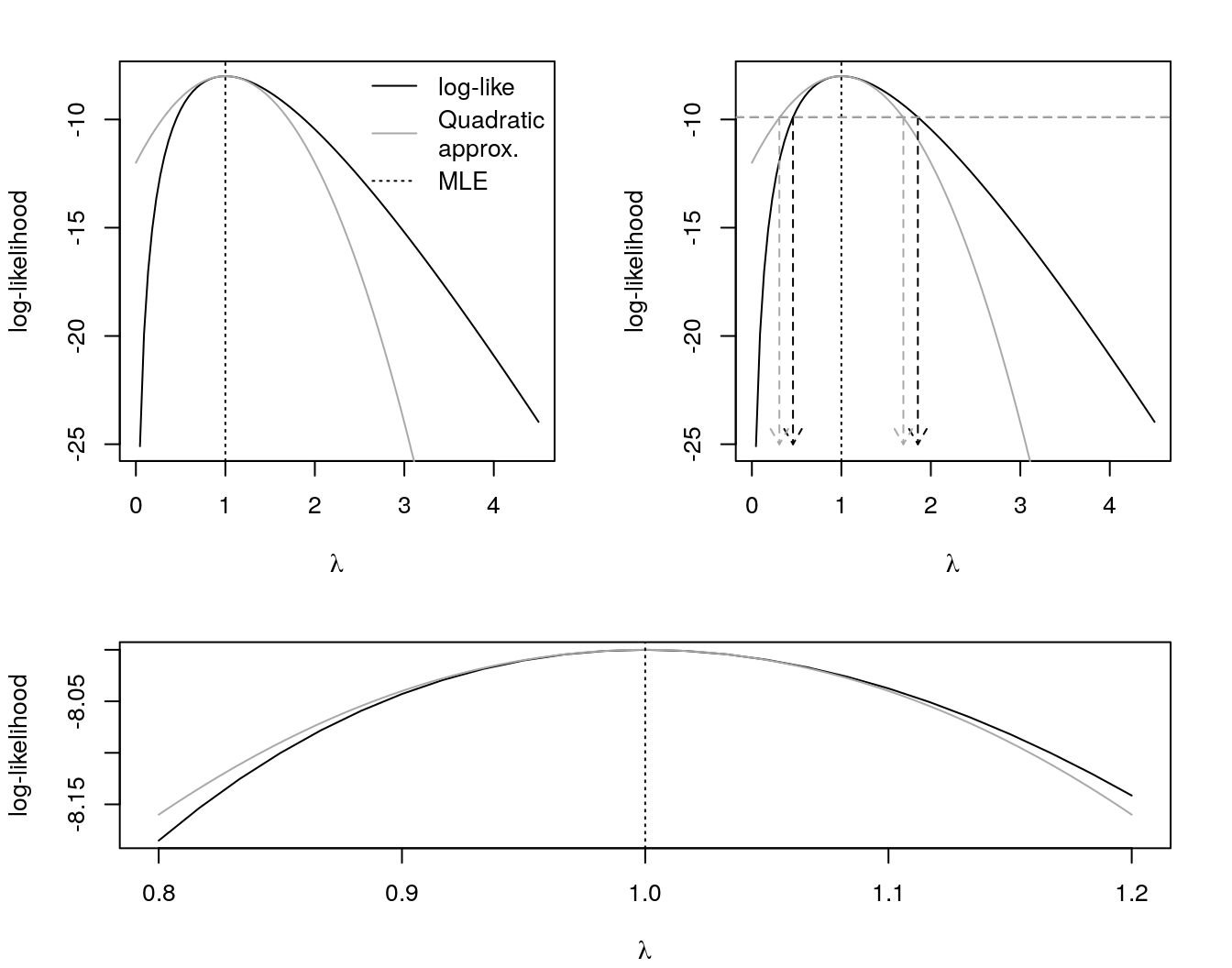
Figure 2: log-likelihood function and MLE of \(\lambda\) in Poisson(\(\lambda\)) based on . In the topleft, a quadratic approximation in gray. In the topright, two intervals for \(\lambda\) - one based in the likelihood (in black) and one based in the quadratic approximation (in gray). In the bottom we provide a better look in the quadratic approximation.
In the topright, in black, we have a interval based in the likelihood, \(\lambda \in (0.459, 1.855)\), but with a cutoff criterion based in a \(\chi^{2}\) distribution. Thus, to have a nominal 95% confidence interval we use a cutoff \(c = 15\%\). As we saw before, this interval is based in a large-sample theory. Since we’re dealing here with a reasonable regular case, this interval shows as a good approximation.
Still in the topright of Figure 2, in red we have a interval based in the quadratic approximation of the log-likelihood, \(\lambda \in (0.307, 1.693)\). From the quadratic approximation we get
\[ \log \frac{L(\lambda)}{L(\hat{\lambda})} \approx -\frac{1}{2} I_{O}(\hat{\lambda}) (\lambda - \hat{\lambda})^{2}, \]
that also follows a \(\chi^{2}\) distribution, since we have a r.v. \(\hat{\lambda}\) normalized (with its expected value subtracted and divided by its variance) and squared. From this we get the following exact (in the normal case) 95% confidence interval
\[ \hat{\lambda} \pm 1.96~I_{O}(\hat{\lambda})^{-1/2} \qquad (\hat{\lambda} \pm 1.96~\text{se}(\hat{\lambda})). \]
In the nonnormal cases this is an approximate 95% CI.
The actual variance is \(I_{E}(\hat{\lambda})^{-1/2}\), but for the Poisson case the Fisher (expected) information is equal to the observed one, \(I_{O}(\hat{\lambda})^{-1/2}\).
A very nice thing that we can see from this intervals is that a Wald interval (a \(\pm\) interval) corresponds to a cut in the quadratic approximation exactly in the same point that the probability-based interval cuts the (log-)likelihood. Thus, as more regular the likelihood, better will be the fit of the approximation and more reliable will be the Wald interval.
Another parametrization
Repeat the previous question for reparametrization \(\theta = \log (\lambda)\).
By the invariance property of the MLE we have
\[ \hat{\lambda} = \bar{x} \quad \Rightarrow \quad g(\hat{\lambda}) = \log \hat{\lambda} = \hat{\theta} = \log \bar{x} = g(\bar{x}). \] i.e., the MLE of \(\hat{\theta}\) is \(\log \bar{x}\).
By the Delta Method we compute the variance of \(\hat{\theta}\),
\[ V[\theta] = V[g(\lambda)] = \left[\frac{\partial}{\partial \lambda} g(\lambda) \right]^{2} V[\lambda] = \left[\frac{1}{\lambda}\right]^{2} \frac{\lambda}{n} = \frac{1}{\lambda~n} \quad \rightarrow \quad V[\hat{\theta}] = \frac{1}{\bar{x}~n}. \] From this we can take the observed information for the reparametrization
\[ V[\hat{\theta}] = I_{O}^{-1}(\hat{\theta}) = (\bar{x}~n)^{-1}. \]
Now we do, in the same manner, everything that we did in the previous letter.
# likelihood ---------------------------------------------------------------------
## we can still use the lkl.poi function, but now we do
## lambda = exp(theta),
## with theta being a real rate (positive or negative)
theta.seq <- seq(-2, 2, length.out = 100)
lklseq.poi <- lkl.poi(exp(theta.seq), data)

par(mar = c(4, 4, 2, 2) + .1)
layout(matrix(c(1, 3, 2, 3), 2, 2), heights = c(1.5, 1)) # plot window definition
plot(theta.seq, lklseq.poi, type = "l",
     xlab = expression(theta), ylab = "log-likelihood")
theta.est <- log(mean(data)) # MLE
abline(v = theta.est, lty = 3)
# quadratic approximation for the reparametrization ------------------------------
quadprox.poi.repa <- function(theta, theta.est, data) {
    obs.info <- sum(data) # observed information
    lkl.poi(exp(theta.est), data) - .5 * obs.info * (theta - theta.est)**2
}
curve(quadprox.poi.repa(x, theta.est, data), col = "darkgray", add = TRUE)

legend(-2.15, -27.5, c("log-like", "Quadratic\napprox.", "MLE"),
       col = c(1, "darkgray", 1), lty = c(1, 1, 3), bty = "n")
# intervals for lambda -----------------------------------------------------------
plot(theta.seq, lklseq.poi, type = "l",
     xlab = expression(theta), ylab = "log-likelihood")
curve(quadprox.poi.repa(x, theta.est, data), col = "darkgray", add = TRUE)
abline(v = theta.est, lty = 3)
## probability-based interval ----------------------------------------------------
# cutoff's corresponding to a 95\% confidence interval for the mean
cut <- log(.15) + lkl.poi(exp(theta.est), data) ; abline(h = cut, lty = 2)
ic.lkl.poi <- function(theta, cut, ...) {
    lambda <- exp(theta)
    lkl.poi(lambda, ...) - cut
}
ic.95.prob <- rootSolve::uniroot.all(ic.lkl.poi, range(theta.seq),
                                     data = data, cut = cut)
arrows(x0 = ic.95.prob, y0 = rep(cut, 2),
       x1 = ic.95.prob, y1 = rep(-43, 2), lty = 2, length = .1)
## wald confidence interval  -----------------------------------------------------
cut <- log(.15) + quadprox.poi.repa(theta.est, theta.est, data)
abline(h = cut, lty = 2, col = "darkgray")

se.theta.est <- sqrt(1 / sum(data))
wald.95 <- theta.est + qnorm(c(.025, .975)) * se.theta.est

arrows(x0 = wald.95, y0 = rep(cut, 2),
       x1 = wald.95, y1 = rep(-43, 2), lty = 2, length = .1, col = "darkgray")
# a better look in the approximation around the MLE ------------------------------
theta.seq <- seq(-.75, .75, length.out = 25)
plot(theta.seq, lkl.poi(exp(theta.seq), data), type = "l",
     xlab = expression(theta), ylab = "log-likelihood")
curve(quadprox.poi.repa(x, theta.est, data), col = "darkgray", add = TRUE)
abline(v = theta.est, lty = 3)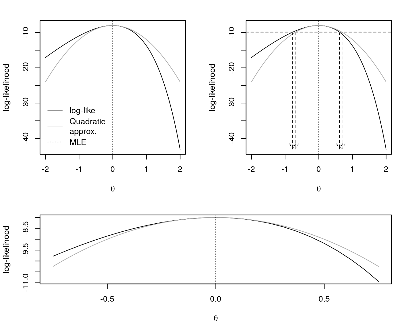
Figure 3: log-likelihood function and MLE of \(\theta\) in Poisson(\(\lambda = e^{\theta}\)) based on . In the topleft, a quadratic approximation in gray. In the topright, two intervals for \(\theta\) - one based in the likelihood (in black) and one based in the quadratic approximation (in gray). In the bottom we provide a better look in the quadratic approximation.
We obtained here two intervals for \(\theta\). One based in a cut in the likelihood, \(\theta \in (-0.778, 0.618)\) - in black on the topright of Figure 3, and one based in a cut in the quadratic approximation of the likelihood, \(\theta \in (`r paste(round(wald.95, 3), collapse = ", ")`)\) - in gray on the topright of Figure 3.
With the parametrization \(\theta = \log \lambda\) the two intervals are closer than the ones obtained for \(\lambda\). i.e., for \(\theta\) (with the use of the \(\log\)) we get a more regular likelihood.
More intervals
Also obtain (by at least two different methods) confidence intervals for the parameter \(\lambda\) from the likelihood function (approximate or not) of \(\theta\).
# likelihood ---------------------------------------------------------------------
theta.seq <- seq(-2, 2, length.out = 100)
lklseq.poi <- lkl.poi(exp(theta.seq), data)

par(mar = c(4, 4, 2, 2) + .1)
plot(theta.seq, lklseq.poi, type = "l",
     xlab = expression(theta), ylab = "log-likelihood")
abline(v = lambda.est, lty = 3)
# quadratic approximation for the reparametrization ------------------------------
curve(quadprox.poi.repa(x, theta.est, data), col = "darkgray", add = TRUE)
legend(-2.15, -25, c("log-like", "Quadratic\napprox.", "MLE"),
       col = c(1, "darkgray", 1), lty = c(1, 1, 3), bty = "n")
# intervals for lambda -----------------------------------------------------------
## probability-based interval ----------------------------------------------------
arrows(x0 = exp(ic.95.prob), y0 = c(-9, -36.5),
       x1 = exp(ic.95.prob), y1 = rep(-43, 2), lty = 2, length = .1)
## wald confidence interval  -----------------------------------------------------
arrows(x0 = exp(wald.95), y0 = c(-9, -24),
       x1 = exp(wald.95), y1 = rep(-43, 2), lty = 2, length = .1, col = "darkgray")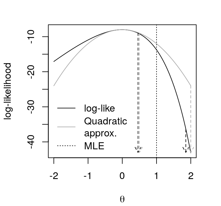
Figure 4: log-likelihood function and quadratic approximation of \(\theta\), and MLE of \(\lambda\) in Poisson(\(\lambda = e^{\theta}\)) based on . In dashed, 95% confidence intervals for \(\lambda\).
Since the MLE has the invariance property, a very simple idea is: take the obtained interval for \(\theta\) and apply a transformation, \(\lambda = e^{\theta}\). This simple idea is true for the interval obtained via likelihood function, as we can see in Figure 4. The obtained interval is the same that the one in letter \(\texttt{a)}\). However, this idea doesn’t work for the interval based in the quadratic approximation.
In the letter \(\texttt{a)}\), via the quadratic approximation we got \(\lambda \in (0.307, 1.693)\). Here, applying the relation \(\lambda = e^{\theta}\) we get \(\lambda \in (0.5, 2)\). i.e., this shows that the invariance property applies to the likelihood, not to the quadratic approximation of the likelihood.