Effect of fungicide sprays programs and pistachio hedging on fruit stain levels caused by Alternaria late blight in commercial pistachio orchard of Tulare County, California
Paulo S. F. Lichtemberg, Ryan D. Puckett, Walmes M. Zeviani, Connor G. Cunningham & Themis J. Michailides
2019-07-11
ake_b-quality.RmdSession Definition
# https://github.com/walmes/wzRfun
# devtools::install_github("walmes/wzRfun")

library(lattice)
library(latticeExtra)
library(plyr)
library(reshape)
library(doBy)
library(multcomp)
library(lme4)
library(lmerTest)
library(wzRfun)library(RDASC)Exploratory data analysis
# Data strucuture.
str(ake_b$quality)
## 'data.frame': 288 obs. of 12 variables:
## $ yr : int 2015 2015 2015 2015 2015 2015 2015 2015 2015 2015 ...
## $ hed: Factor w/ 2 levels "heavy","normal": 1 1 1 1 1 1 1 1 1 1 ...
## $ tra: Factor w/ 4 levels "cnt","fon2","mer2",..: 4 4 4 4 4 4 4 4 4 1 ...
## $ plo: Factor w/ 12 levels "1A","1B","1C",..: 1 1 1 1 1 1 1 1 1 1 ...
## $ tre: int 1 1 1 2 2 2 3 3 3 4 ...
## $ rep: int 1 2 3 1 2 3 1 2 3 1 ...
## $ c0 : int 2 4 7 4 0 0 0 0 2 NA ...
## $ c1 : int 27 55 53 31 44 38 22 21 25 NA ...
## $ c2 : int 18 12 12 26 40 37 25 32 36 NA ...
## $ c3 : int 16 16 14 33 8 18 19 12 15 NA ...
## $ c4 : int 37 13 14 6 8 7 34 35 22 NA ...
## $ tot: int 100 100 100 100 100 100 100 100 100 NA ...# Short names are easier to use.
da <- ake_b$quality
da$yr <- factor(da$yr)
intlev <- c(c0 = "[0]",
c1 = "[1, 10]",
c2 = "[11, 35]",
c3 = "[36, 64]",
c4 = "[65, 100]")
# Creating the blocks.
da$block <- with(da, {
factor(ifelse(as.integer(gsub("\\D", "", plo)) > 2, "II", "I"))
})
# Creating unique levels for trees.
da$tre <- with(da,
interaction(hed, tra, block, tre, drop = TRUE))
# Stack data to plot variables.
db <- melt(da,
id.vars = 1:6,
measure.vars = grep("c\\d", names(ake_b$quality)),
na.rm = TRUE)
names(db)[ncol(db) - 1:0] <- c("categ", "freq")
useOuterStrips(
xyplot(freq ~ categ | hed + yr,
groups = tra,
data = db,
xlab = "Percentage of the shell surface discolored",
ylab = "Number of fruits in each class (n = 100)",
jitter.x = TRUE,
scales = list(x = list(labels = intlev,
alternating = 1)),
auto.key = list(columns = 2,
title = "Fungicide",
cex.title = 1.1),
type = c("p", "a")))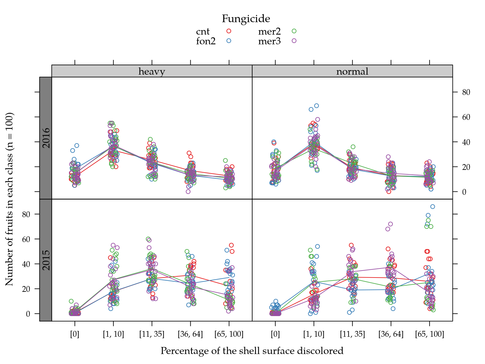
useOuterStrips(
    xyplot(freq ~ categ | tra + yr,
           groups = hed,
           data = db,
           xlab = "Percentage of the shell surface discolored",
           ylab = "Number of fruits in each class (n = 100)",
           jitter.x = TRUE,
           scales = list(x = list(labels = intlev,
                                  rot = 45,
                                  alternating = 1)),
           auto.key = list(columns = 2,
                           title = "Hed",
                           cex.title = 1.1),
           type = c("p", "a")))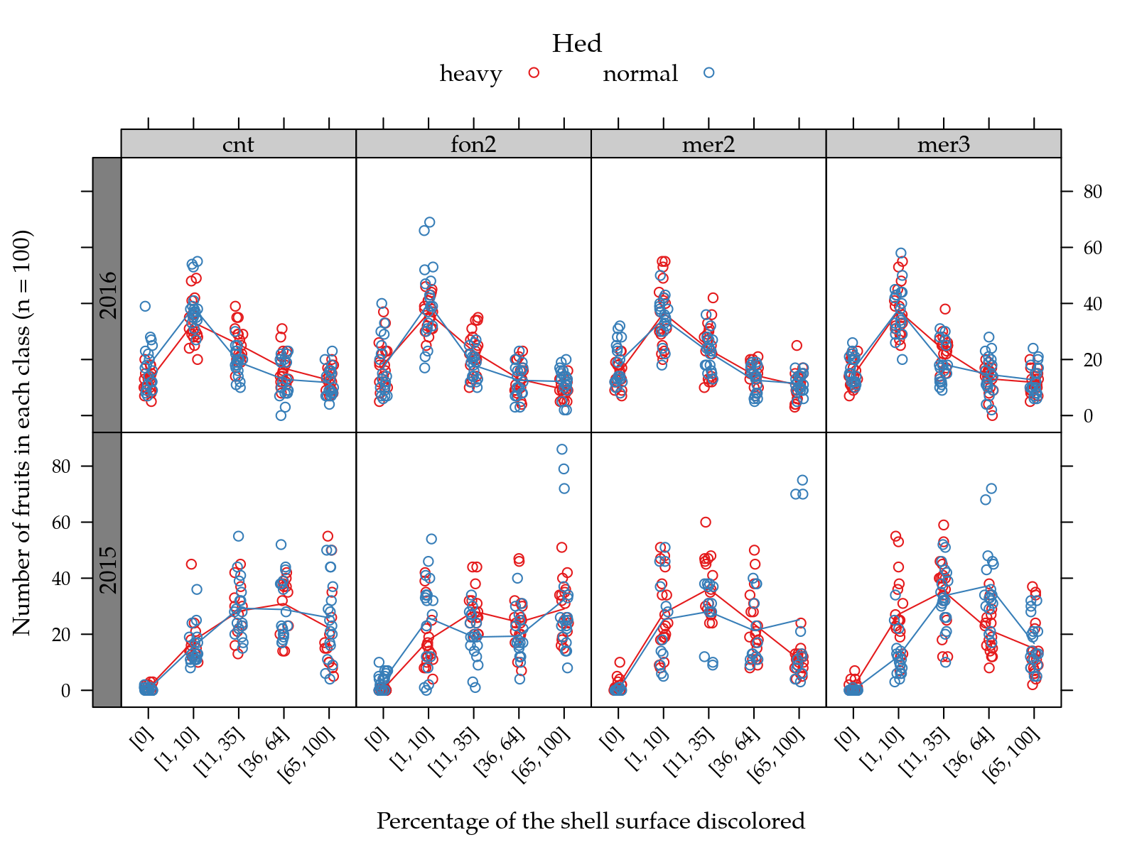
i <- grep("^c\\d$", x = names(da))

# useOuterStrips(
#     splom(~da[, i] | hed + yr,
#           groups = tra,
#           type = c("p", "r"),
#           data = da))
# Acumulated proportion.
cml <- t(apply(da[, i], MARGIN = 1, FUN = cumsum))
cml <- cml[, -length(i)]
colnames(cml) <- paste0("p", 1:ncol(cml))
# Add acummulated proportions.
da <- cbind(da, as.data.frame(cml))
db <- melt(da,
id.vars = 1:6,
measure.vars = colnames(cml),
na.rm = TRUE)
names(db)[ncol(db) - 1:0] <- c("categ", "prop")
str(db)## 'data.frame': 1104 obs. of 8 variables:
## $ yr : Factor w/ 2 levels "2015","2016": 1 1 1 1 1 1 1 1 1 1 ...
## $ hed : Factor w/ 2 levels "heavy","normal": 1 1 1 1 1 1 1 1 1 2 ...
## $ tra : Factor w/ 4 levels "cnt","fon2","mer2",..: 4 4 4 4 4 4 4 4 4 2 ...
## $ plo : Factor w/ 12 levels "1A","1B","1C",..: 1 1 1 1 1 1 1 1 1 2 ...
## $ tre : Factor w/ 48 levels "heavy.mer3.I.1",..: 1 1 1 2 2 2 3 3 3 5 ...
## $ rep : int 1 2 3 1 2 3 1 2 3 1 ...
## $ categ: Factor w/ 4 levels "p1","p2","p3",..: 1 1 1 1 1 1 1 1 1 1 ...
## $ prop : int 2 4 7 4 0 0 0 0 2 0 ...accumlev <- c(p1 = "0",
p2 = "<=10",
p3 = "<=35",
p4 = "<=65")
useOuterStrips(
xyplot(prop ~ categ | hed + yr,
groups = tra,
data = db,
xlab = "Percentage of the shell surface discolored",
ylab = "Number of fruits in each class (n = 100)",
jitter.x = TRUE,
auto.key = list(columns = 2,
title = "Fungicide",
cex.title = 1.1),
scales = list(x = list(labels = accumlev,
alternating = 1)),
type = c("p", "a")))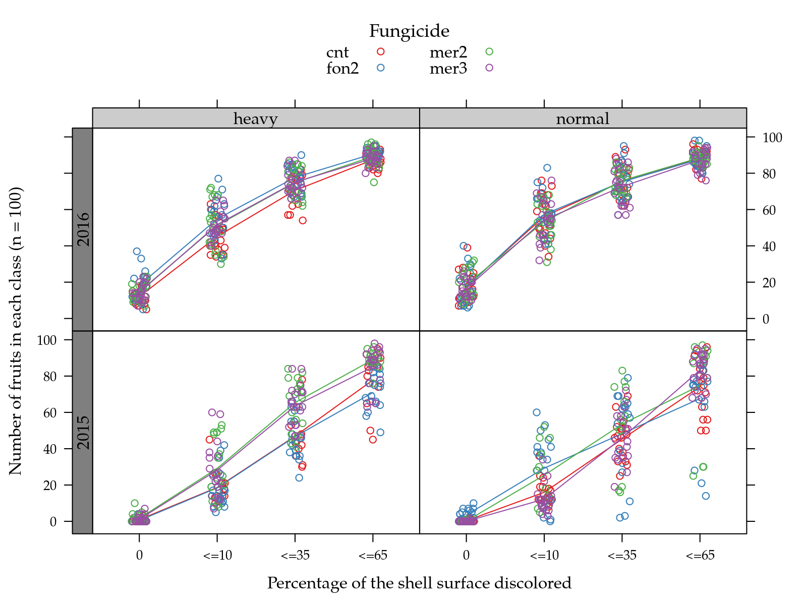
useOuterStrips(
    xyplot(prop ~ categ | tra + yr,
           groups = hed,
           data = db,
           xlab = "Percentage of the shell surface discolored",
           ylab = "Number of fruits in each category (n = 100)",
           jitter.x = TRUE,
           auto.key = list(columns = 2,
                           title = "Hed",
                           cex.title = 1.1),
           scales = list(x = list(labels = accumlev,
                                  alternating = 1)),
           type = c("p", "a")))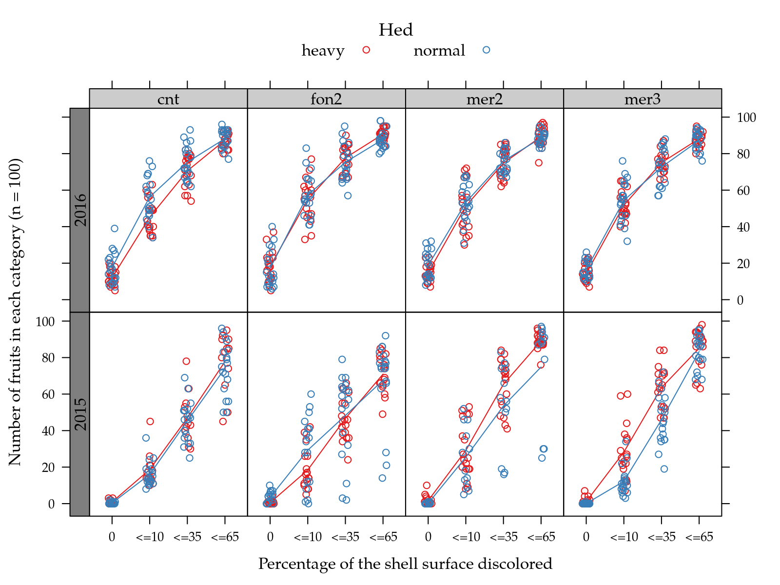
Analysis of the accumulated proportion
The plots above showed that the greatest difference among levels of treaments, either hed or fungicides, occurs for the accumulated proportions at class \(\leq 35\) (p2). Because of this, the analysis will be for this response variable.
The total number of independent observations results from the calculus \[ \begin{aligned} 288 \text{ observations} &= 2 \text{ years } \times 2 \text{ blocks } \times \\ &\quad\,\, 2 \text{ heds } \times 4 \text{ fungicides } \times \\ &\quad\,\, 3 \text{ trees } \times 3 \text{ bags}.\\ \end{aligned} \]
da$y <- da$p2
da <- da[!is.na(da$y), ]

xyplot(p2 ~ tra | yr,
       groups = hed,
       data = da,
       type = c("p", "a"),
       xlab = "Fungicides",
       ylab = expression("Number of fruits with" <= "35% of the shell surface discolored"),
       jitter.x = TRUE,
       auto.key = list(columns = 2,
                       title = "Hed",
                       cex.title = 1.1))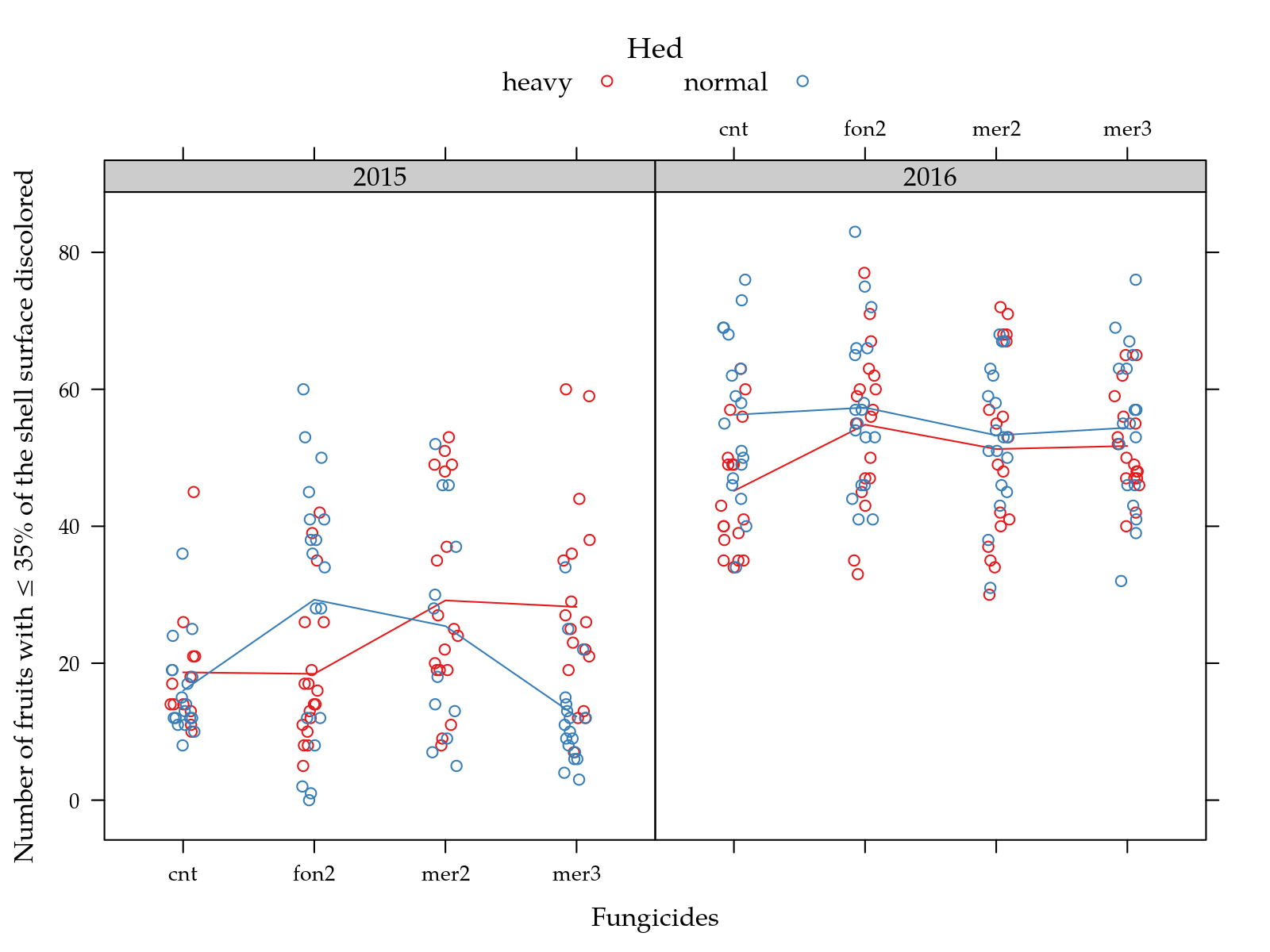
Figure 1: Number of fruits with 35% or less of the shell surface discolored as a function of the fungicide and hed level for two years.
# xyplot(p2 ~ yr | tre,
#        data = da,
#        xlab = "Years",
#        ylab = "Number of fruits with 35% or less damage",
#        as.table = TRUE,
#        jitter.x = TRUE)
The analysis are being separated for each year. First, although the choosen response variable is limited or bounded (because it is a sample proportion), it doesn’t show problematic departures from a linear (gaussian) model. Linear models are more flexible for analysing clutered data as such.
da15 <- subset(da, yr == "2015")
da16 <- subset(da, yr == "2016")

# Quasi-binomial model.
# m0 <- glm(cbind(p2, 100 - p2) ~ block + yr * hed * tra,
#           family = quasibinomial,
#           data = da)

# Just to check if the model assumptions are meet.
m0 <- lm(p2 ~ block + yr * hed * tra,
         data = da)
par(mfrow = c(2, 2))
plot(m0); layout(1)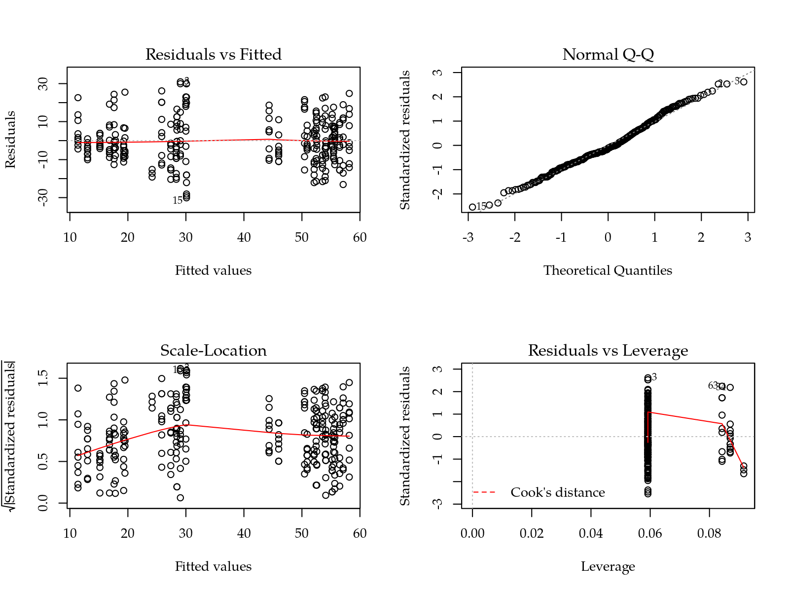
# Normal approximation goes well.A simple linear models is fitted only to check how the residuals behave. No evidence of departures from models assumptions were found.
# Year 2015.
m15 <- lmer(p2 ~ block + hed * tra + (1 | tre),
           data = da15)

# r <- residuals(m15)
# f <- fitted(m15)
# plot(r ~ f)
# qqnorm(r)

anova(m15)
## Type III Analysis of Variance Table with Satterthwaite's method
## Sum Sq Mean Sq NumDF DenDF F value Pr(>F)
## block 32.467 32.467 1 35 1.0525 0.3120
## hed 18.445 18.445 1 35 0.5979 0.4446
## tra 87.850 29.283 3 35 0.9493 0.4274
## hed:tra 189.773 63.258 3 35 2.0506 0.1246summary(m15)## Linear mixed model fit by REML. t-tests use Satterthwaite's method
## [lmerModLmerTest]
## Formula: p2 ~ block + hed * tra + (1 | tre)
## Data: da15
##
## REML criterion at convergence: 896.2
##
## Scaled residuals:
## Min 1Q Median 3Q Max
## -3.4619 -0.4981 -0.1348 0.5054 2.6844
##
## Random effects:
## Groups Name Variance Std.Dev.
## tre (Intercept) 166.72 12.912
## Residual 30.85 5.554
## Number of obs: 132, groups: tre, 44
##
## Fixed effects:
## Estimate Std. Error df t value Pr(>|t|)
## (Intercept) 20.7481 6.9546 34.9999 2.983 0.00517 **
## blockII -4.1628 4.0577 34.9999 -1.026 0.31198
## hednormal -2.6667 8.5878 34.9999 -0.311 0.75801
## trafon2 -0.2222 8.5878 34.9999 -0.026 0.97950
## tramer2 10.5000 8.5878 34.9999 1.223 0.22962
## tramer3 9.5556 8.5878 34.9999 1.113 0.27342
## hednormal:trafon2 13.5000 11.5217 34.9999 1.172 0.24923
## hednormal:tramer2 -2.1240 12.1872 34.9999 -0.174 0.86265
## hednormal:tramer3 -13.3333 11.5217 34.9999 -1.157 0.25501
## ---
## Signif. codes: 0 '***' 0.001 '**' 0.01 '*' 0.05 '.' 0.1 ' ' 1
##
## Correlation of Fixed Effects:
## (Intr) blckII hdnrml trafn2 tramr2 tramr3 hdnrml:trf2
## blockII -0.292
## hednormal -0.741 0.000
## trafon2 -0.741 0.000 0.600
## tramer2 -0.741 0.000 0.600 0.600
## tramer3 -0.741 0.000 0.600 0.600 0.600
## hdnrml:trf2 0.552 0.000 -0.745 -0.745 -0.447 -0.447
## hdnrml:trm2 0.498 0.083 -0.705 -0.423 -0.705 -0.423 0.525
## hdnrml:trm3 0.552 0.000 -0.745 -0.447 -0.447 -0.745 0.556
## hdnrml:trm2
## blockII
## hednormal
## trafon2
## tramer2
## tramer3
## hdnrml:trf2
## hdnrml:trm2
## hdnrml:trm3 0.525# Year 2016.
m16 <- lmer(p2 ~ block + hed * tra + (1 | tre),
data = da16)
# r <- residuals(m16)
# f <- fitted(m16)
# plot(r ~ f)
# qqnorm(r)
anova(m16)## Type III Analysis of Variance Table with Satterthwaite's method
## Sum Sq Mean Sq NumDF DenDF F value Pr(>F)
## block 1.385 1.385 1 39 0.0374 0.8476
## hed 81.092 81.092 1 39 2.1913 0.1468
## tra 59.092 19.697 3 39 0.5323 0.6629
## hed:tra 55.633 18.544 3 39 0.5011 0.6837summary(m16)## Linear mixed model fit by REML. t-tests use Satterthwaite's method
## [lmerModLmerTest]
## Formula: p2 ~ block + hed * tra + (1 | tre)
## Data: da16
##
## REML criterion at convergence: 984.2
##
## Scaled residuals:
## Min 1Q Median 3Q Max
## -2.06240 -0.61593 -0.05643 0.60353 1.87718
##
## Random effects:
## Groups Name Variance Std.Dev.
## tre (Intercept) 102.01 10.100
## Residual 37.01 6.083
## Number of obs: 144, groups: tre, 48
##
## Fixed effects:
## Estimate Std. Error df t value Pr(>|t|)
## (Intercept) 44.8681 4.6303 39.0000 9.690 6.19e-12 ***
## blockII 0.5972 3.0869 39.0000 0.193 0.8476
## hednormal 11.1111 6.1737 39.0000 1.800 0.0796 .
## trafon2 9.6667 6.1737 39.0000 1.566 0.1255
## tramer2 6.1111 6.1737 39.0000 0.990 0.3283
## tramer3 6.5556 6.1737 39.0000 1.062 0.2948
## hednormal:trafon2 -8.6111 8.7309 39.0000 -0.986 0.3301
## hednormal:tramer2 -9.1111 8.7309 39.0000 -1.044 0.3031
## hednormal:tramer3 -8.4444 8.7309 39.0000 -0.967 0.3394
## ---
## Signif. codes: 0 '***' 0.001 '**' 0.01 '*' 0.05 '.' 0.1 ' ' 1
##
## Correlation of Fixed Effects:
## (Intr) blckII hdnrml trafn2 tramr2 tramr3 hdnrml:trf2
## blockII -0.333
## hednormal -0.667 0.000
## trafon2 -0.667 0.000 0.500
## tramer2 -0.667 0.000 0.500 0.500
## tramer3 -0.667 0.000 0.500 0.500 0.500
## hdnrml:trf2 0.471 0.000 -0.707 -0.707 -0.354 -0.354
## hdnrml:trm2 0.471 0.000 -0.707 -0.354 -0.707 -0.354 0.500
## hdnrml:trm3 0.471 0.000 -0.707 -0.354 -0.354 -0.707 0.500
## hdnrml:trm2
## blockII
## hednormal
## trafon2
## tramer2
## tramer3
## hdnrml:trf2
## hdnrml:trm2
## hdnrml:trm3 0.500For both years, no effect were found for the experimental factors.
# Represent the results with interval confidence on ls means.
cmp <- list()

lsm <- LSmeans(m15, effect = "hed")
grid <- equallevels(lsm$grid, da)

L <- lsm$L
rownames(L) <- grid[, 1]

cmp$hed <-
    rbind(
        cbind(yr = "2015", apmc(L, model = m15, focus = "hed")),
        cbind(yr = "2016", apmc(L, model = m16, focus = "hed")))

lsm <- LSmeans(m15, effect = "tra")
grid <- equallevels(lsm$grid, da)

L <- lsm$L
rownames(L) <- grid[, 1]

cmp$tra <-
    rbind(
        cbind(yr = "2015", apmc(L, model = m15, focus = "tra")),
        cbind(yr = "2016", apmc(L, model = m16, focus = "tra")))

cmp <- ldply(cmp,
             .id = "effect",
             .fun = function(x) {
                 names(x)[2] <- "level"
                 return(x)
             })
cmp$level <- factor(cmp$level, levels = unique(cmp$level))
cmp
## effect yr level fit lwr upr cld
## 1 hed 2015 heavy 23.62500 17.979480 29.27052 a
## 2 hed 2015 normal 20.46899 14.801633 26.13635 a
## 3 hed 2016 heavy 50.75000 46.471921 55.02808 a
## 4 hed 2016 normal 55.31944 51.041366 59.59752 a
## 5 tra 2015 cnt 17.33333 8.917489 25.74918 a
## 6 tra 2015 fon2 23.86111 16.333751 31.38847 a
## 7 tra 2015 mer2 26.77132 18.296962 35.24567 a
## 8 tra 2015 mer3 20.22222 12.694862 27.74958 a
## 9 tra 2016 cnt 50.72222 44.672105 56.77234 a
## 10 tra 2016 fon2 56.08333 50.033216 62.13345 a
## 11 tra 2016 mer2 52.27778 46.227661 58.32790 a
## 12 tra 2016 mer3 53.05556 47.005438 59.10567 aresizePanels(
useOuterStrips(
segplot(level ~ lwr + upr | yr + effect,
centers = fit,
data = cmp,
draw = FALSE,
xlab = "Proportion of fruits with 35% or less damage",
ylab = "Levels of the factors",
scales = list(y = list(relation = "free"),
alternating = 1),
ann = sprintf("%0.2f %s", cmp$fit, cmp$cld)
)
), h = c(2, 4)) +
layer(panel.text(x = centers[subscripts],
y = z[subscripts],
labels = ann[subscripts],
pos = 3))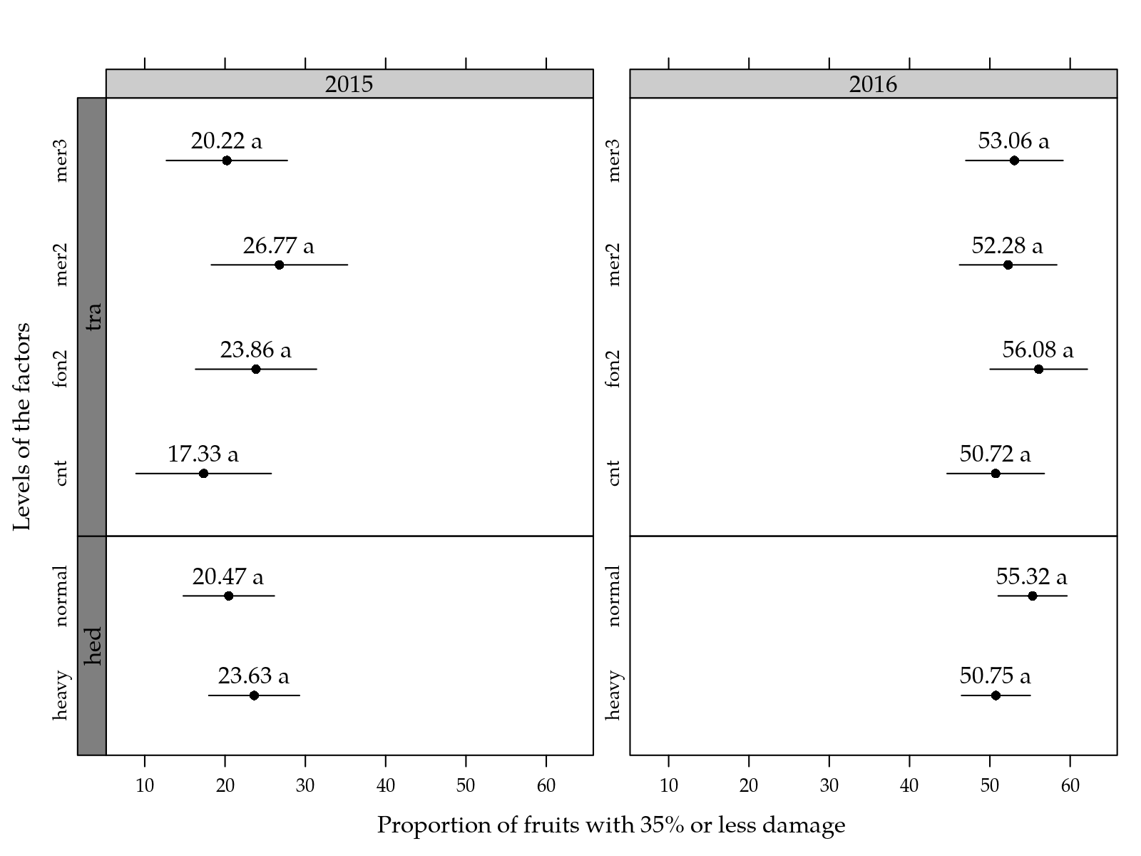
Figure 2: Mean proportion of fruits with 35% or less of the shell surface discolored as a function of the fungicide and hed level for two years.
Session information
## quinta, 11 de julho de 2019, 20:03
## ----------------------------------------
## R version 3.6.1 (2019-07-05)
## Platform: x86_64-pc-linux-gnu (64-bit)
## Running under: Ubuntu 18.04.2 LTS
##
## Matrix products: default
## BLAS:   /usr/lib/x86_64-linux-gnu/blas/libblas.so.3.7.1
## LAPACK: /usr/lib/x86_64-linux-gnu/lapack/liblapack.so.3.7.1
##
## locale:
##  [1] LC_CTYPE=pt_BR.UTF-8       LC_NUMERIC=C
##  [3] LC_TIME=pt_BR.UTF-8        LC_COLLATE=en_US.UTF-8
##  [5] LC_MONETARY=pt_BR.UTF-8    LC_MESSAGES=en_US.UTF-8
##  [7] LC_PAPER=pt_BR.UTF-8       LC_NAME=C
##  [9] LC_ADDRESS=C               LC_TELEPHONE=C
## [11] LC_MEASUREMENT=pt_BR.UTF-8 LC_IDENTIFICATION=C
##
## attached base packages:
## [1] stats     graphics  grDevices utils     datasets  methods
## [7] base
##
## other attached packages:
##  [1] captioner_2.2.3     knitr_1.23          RDASC_0.0-6
##  [4] wzRfun_0.81         lmerTest_3.1-0      lme4_1.1-21
##  [7] Matrix_1.2-17       multcomp_1.4-10     TH.data_1.0-10
## [10] MASS_7.3-51.4       survival_2.44-1.1   mvtnorm_1.0-11
## [13] doBy_4.6-2          reshape_0.8.8       plyr_1.8.4
## [16] latticeExtra_0.6-28 RColorBrewer_1.1-2  lattice_0.20-38
##
## loaded via a namespace (and not attached):
##  [1] zoo_1.8-6           tidyselect_0.2.5    xfun_0.8
##  [4] purrr_0.3.2         splines_3.6.1       tcltk_3.6.1
##  [7] colorspace_1.4-1    htmltools_0.3.6     rpanel_1.1-4
## [10] yaml_2.2.0          rlang_0.4.0         pkgdown_1.3.0
## [13] pillar_1.4.2        nloptr_1.2.1        glue_1.3.1
## [16] stringr_1.4.0       munsell_0.5.0       commonmark_1.7
## [19] gtable_0.3.0        codetools_0.2-16    memoise_1.1.0
## [22] evaluate_0.14       parallel_3.6.1      pbkrtest_0.4-7
## [25] highr_0.8           Rcpp_1.0.1          backports_1.1.4
## [28] scales_1.0.0        desc_1.2.0          fs_1.3.1
## [31] ggplot2_3.2.0       digest_0.6.20       stringi_1.4.3
## [34] dplyr_0.8.3         numDeriv_2016.8-1.1 grid_3.6.1
## [37] rprojroot_1.3-2     tools_3.6.1         sandwich_2.5-1
## [40] magrittr_1.5        lazyeval_0.2.2      tibble_2.1.3
## [43] crayon_1.3.4        pkgconfig_2.0.2     xml2_1.2.0
## [46] assertthat_0.2.1    minqa_1.2.4         rmarkdown_1.13
## [49] roxygen2_6.1.1      R6_2.4.0            boot_1.3-23
## [52] nlme_3.1-140        compiler_3.6.1