Curva de retenção de Água na Cultura do Abacaxizeiro em Função da Cobertura do Solo e Aplicação de Gesso
Walmes Zeviani & Milson Evaldo Serafim
2019-07-11
pineapple_swrc.RmdDefinições da sessão
# https://github.com/walmes/wzRfun
# devtools::install_github("walmes/wzRfun")
library(wzRfun)

pkg <- c("lattice",
         "latticeExtra",
         "nlme",
         "reshape",
         "plyr",
         "doBy",
         "multcomp")
sapply(pkg, library, character.only = TRUE, logical.return = TRUE)library(RDASC)Importação dos dados
#-----------------------------------------------------------------------
# Lendo arquivos de dados.

data(pineapple_swrc)
str(pineapple_swrc)
## 'data.frame': 1662 obs. of 7 variables:
## $ cober: Factor w/ 2 levels "Millet","No millet": 1 1 1 1 1 1 1 1 1 1 ...
## $ gesso: int 0 0 0 0 0 0 0 0 0 0 ...
## $ prof : Factor w/ 2 levels "0-0.05","0.05-0.20": 1 1 1 1 1 1 1 1 1 1 ...
## $ varie: Factor w/ 4 levels "IAC Fantastico",..: 3 3 3 3 3 3 3 3 3 3 ...
## $ bloc : int 1 2 3 4 1 2 3 4 1 2 ...
## $ tens : int 0 0 0 0 1 1 1 1 2 2 ...
## $ umid : num 0.488 0.433 0.343 0.415 0.489 ...# Converte variáveis para fator.
pineapple_swrc <-
transform(pineapple_swrc,
gesso = factor(gesso),
ue = interaction(cober, gesso, prof, varie, bloc,
drop = TRUE, sep = ":"))
# Passa a tensão 0 para 0.01 para não ter problemas com o log().
pineapple_swrc$tens[pineapple_swrc$tens == 0] <- 0.01
pineapple_swrc$ltens <- log10(pineapple_swrc$tens)
# Mostra a estrutura do objeto.
str(pineapple_swrc)## 'data.frame': 1662 obs. of 9 variables:
## $ cober: Factor w/ 2 levels "Millet","No millet": 1 1 1 1 1 1 1 1 1 1 ...
## $ gesso: Factor w/ 2 levels "0","4": 1 1 1 1 1 1 1 1 1 1 ...
## $ prof : Factor w/ 2 levels "0-0.05","0.05-0.20": 1 1 1 1 1 1 1 1 1 1 ...
## $ varie: Factor w/ 4 levels "IAC Fantastico",..: 3 3 3 3 3 3 3 3 3 3 ...
## $ bloc : int 1 2 3 4 1 2 3 4 1 2 ...
## $ tens : num 0.01 0.01 0.01 0.01 1 1 1 1 2 2 ...
## $ umid : num 0.488 0.433 0.343 0.415 0.489 ...
## $ ue : Factor w/ 128 levels "Millet:0:0-0.05:IAC Fantastico:1",..: 17 49 81 113 17 49 81 113 17 49 ...
## $ ltens: num -2 -2 -2 -2 0 ...Análise exploratória
#-----------------------------------------------------------------------
# Análise exploratória.

# Identifica as unidades com a combinação tripla dos fatores.
pineapple_swrc$gescobpro <-
    with(pineapple_swrc, interaction(as.integer(gesso),
                                     as.integer(cober),
                                     as.integer(prof)))

p1 <- xyplot(umid ~ tens | gescobpro + varie,
             data = pineapple_swrc,
             groups = bloc, type = "b",
             ylab = "Moisture",
             xlab = "log 10 of matric tension",
             scales = list(x = list(log = 10)),
             xscale.components = xscale.components.log10ticks)
useOuterStrips(p1)
# Número de curvas.
nlevels(pineapple_swrc$ue)
## [1] 128#-----------------------------------------------------------------------
# Identificar os pontos atípicos.
# i <- 1:nrow(pineapple_swrc)
# useOuterStrips(p1)
# panel.locs <- trellis.currentLayout()
# outliers <- vector(mode = "list",
# length = prod(dim(panel.locs)))
# for (row in 1:nrow(panel.locs)) {
# for (column in 1:ncol(panel.locs)) {
# if (panel.locs[row, column] > 0) {
# trellis.focus("panel",
# row = row,
# column = column,
# highlight = TRUE)
# wp <- panel.locs[row, column]
# obsv <- panel.identify()
# # print(obsv)
# j <- column + (row - 1) * nrow(panel.locs)
# # print(j)
# outliers[[j]] <- i[obsv]
# trellis.unfocus()
# }
# }
# }
# Clicar com o botão direito em cada cela (de baixo para cima, esquerda
# para direita) para identificar o ponto outliear. Clicar com o botão
# direito para passara para a próxima cela.
# outliers
# r <- unlist(outliers)
# dput(r)
# Outiliers identificados visualmente.
out <- c(106L, 151L, 1397L, 513L, 717L, 725L)
pineapple_swrc <- pineapple_swrc[-out, ]Ajuste de forma interativa
#-----------------------------------------------------------------------
# Ajuste com rp.nls.

model <- umid ~ Ur + (Us - Ur)/(1 + exp(n * (alp + ltens)))^(1 - 1/n)
start <- list(Ur = c(0.1,   0, 0.4),
              Us = c(0.4, 0.1, 0.8),
              alp =c(1,    -5,   6),
              n =  c(1.5,   1,   4))

library(rpanel)

cra.fit <- rp.nls(model = model,
                  data = pineapple_swrc,
                  start = start)

summary(cra.fit)
Ajuste por unidade experimental
O ajuste foi feito considerando a seguinte parametrização do modelo van Genuchten
\[ U(x) = U_r + \frac{U_s - U_r}{(1 + \exp\{n(\alpha + x)\})^{1 - 1/n}} \]
em que \(U\) é umidade (m3 m-3) do solo, \(x\) é o log na base 10 da tensão matricial aplicada (kPa), \(U_r\) é a umidade residual (assíntota inferior), \(U_s\) é a umidade de satuação (assíntota superior), \(\alpha\) e \(n\) são parâmetros empíricos de forma da curva de retenção de água. Uma vez conhecido valores para as quatidades mencionadas, são obtidos
\[ \begin{align*} S &= -n\cdot \frac{U_s - U_r}{(1 + 1/m)^{m + 1}} \newline I &= -\alpha - \log(m)/n \newline U_I &= U(x = I) \end{align*} \]
em que \(S\) é a taxa no ponto de inflexão, parâmetro que é tido como central para avaliação da qualidade física do solo, bem como \(I\) que corresponde ao log da tensão no ponto de inflexão da curva de retenção de água do solo. A umidade correspondente a tensão no ponto de inflexão é representada por \(U_I\).
#-----------------------------------------------------------------------
# Ajustar uma única curva.

model <- umid ~ Ur + (Us - Ur)/(1 + exp(n * (alp + ltens)))^(1 - 1/n)
start <- list(Ur = 0.1, Us = 0.4, alp = -0.5, n = 4)

plot(umid ~ ltens, data = pineapple_swrc)
with(start, curve(Ur + (Us - Ur)/(1 + exp(n * (alp + x)))^(1 - 1/n),
                  add = TRUE))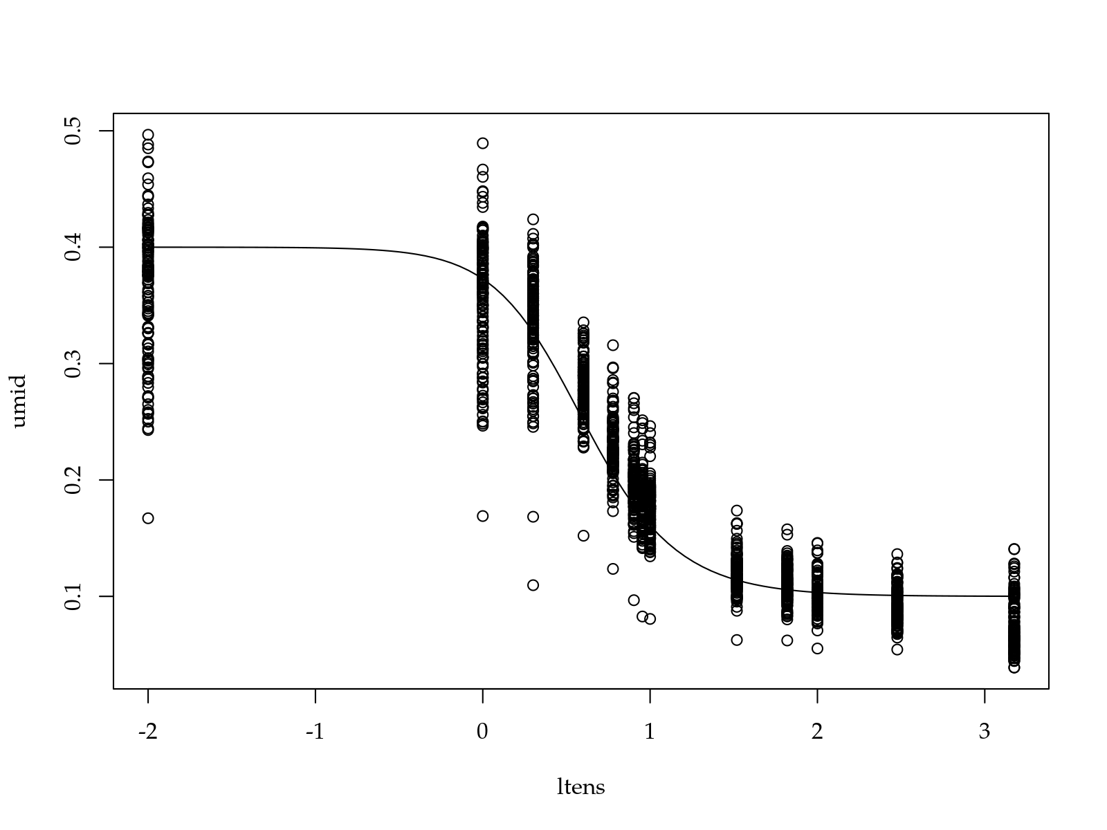
##          Ur          Us         alp           n
##  0.09186589  0.36666033 -0.68298513  4.05581675
#-----------------------------------------------------------------------
# Ajudar para cada unidade experimental.
# nlevels(pineapple_swrc$ue)
db <- groupedData(umid ~ ltens | ue,
data = pineapple_swrc, order.groups = FALSE)
str(db)## Classes 'nfnGroupedData', 'nfGroupedData', 'groupedData' and 'data.frame': 1656 obs. of 10 variables:
## $ cober : Factor w/ 2 levels "Millet","No millet": 1 1 1 1 1 1 1 1 1 1 ...
## $ gesso : Factor w/ 2 levels "0","4": 1 1 1 1 1 1 1 1 1 1 ...
## $ prof : Factor w/ 2 levels "0-0.05","0.05-0.20": 1 1 1 1 1 1 1 1 1 1 ...
## $ varie : Factor w/ 4 levels "IAC Fantastico",..: 3 3 3 3 3 3 3 3 3 3 ...
## $ bloc : int 1 2 3 4 1 2 3 4 1 2 ...
## $ tens : num 0.01 0.01 0.01 0.01 1 1 1 1 2 2 ...
## $ umid : num 0.488 0.433 0.343 0.415 0.489 ...
## $ ue : Factor w/ 128 levels "Millet:0:0-0.05:IAC Fantastico:1",..: 17 49 81 113 17 49 81 113 17 49 ...
## $ ltens : num -2 -2 -2 -2 0 ...
## $ gescobpro: Factor w/ 8 levels "1.1.1","2.1.1",..: 1 1 1 1 1 1 1 1 1 1 ...
## - attr(*, "formula")=Class 'formula' language umid ~ ltens | ue
## .. ..- attr(*, ".Environment")=<environment: R_GlobalEnv>
## - attr(*, "FUN")=function (x)
## - attr(*, "order.groups")= logi FALSEn0 <- nlsList(model = model,
data = db,
start = as.list(coef(n00)))
c0 <- coef(n0)
# Matriz de diagramas de dispersão.
pairs(c0)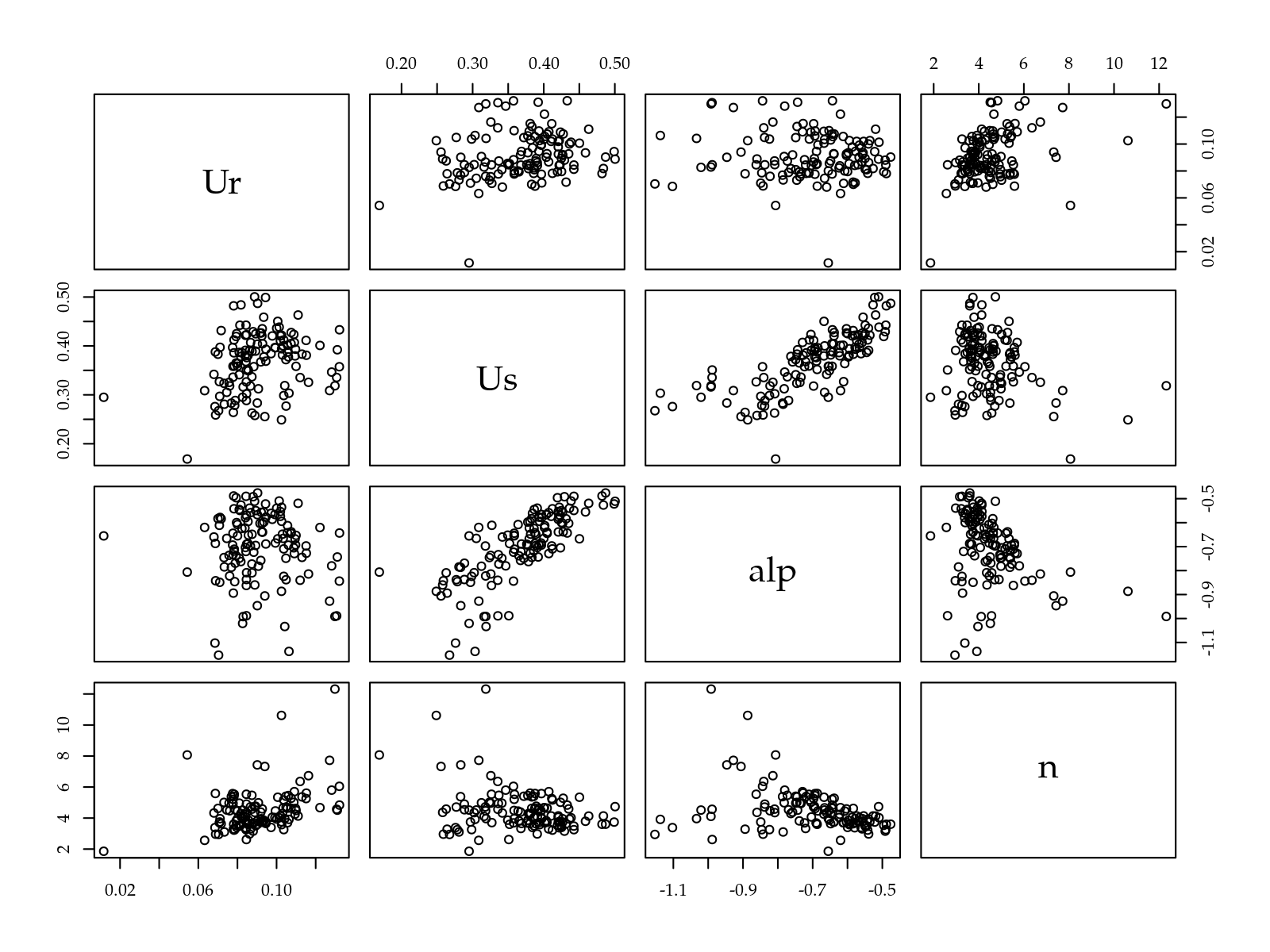
#-----------------------------------------------------------------------
# Correr análises de variância considerando parâmetros como variáveis
# resposta.

aux <- do.call(rbind, strsplit(rownames(c0), split = ":"))
colnames(aux) <- c("cober", "gesso", "prof", "varie", "bloc")
params <- cbind(equallevels(as.data.frame(aux), pineapple_swrc), c0)
rownames(params) <- NULL
str(params)
## 'data.frame': 128 obs. of 9 variables:
## $ cober: Factor w/ 2 levels "Millet","No millet": 1 2 1 2 1 2 1 2 1 2 ...
## $ gesso: Factor w/ 2 levels "0","4": 1 1 2 2 1 1 2 2 1 1 ...
## $ prof : Factor w/ 2 levels "0-0.05","0.05-0.20": 1 1 1 1 2 2 2 2 1 1 ...
## $ varie: Factor w/ 4 levels "IAC Fantastico",..: 1 1 1 1 1 1 1 1 2 2 ...
## $ bloc : Factor w/ 4 levels "1","2","3","4": 1 1 1 1 1 1 1 1 1 1 ...
## $ Ur : num 0.104 0.068 0.094 0.103 0.115 ...
## $ Us : num 0.412 0.342 0.256 0.382 0.381 ...
## $ alp : num -0.709 -0.66 -0.906 -0.648 -0.727 ...
## $ n : num 5.17 4.33 7.33 4.29 5.61 ...#-----------------------------------------------------------------------
# Manova.
m0 <- aov(cbind(Ur, Us, n, alp) ~ cober * gesso * prof * varie,
data = params)
anova(m0)## Analysis of Variance Table
##
## Df Pillai approx F num Df den Df Pr(>F)
## (Intercept) 1 0.99725 8436.8 4 93 < 2.2e-16
## cober 1 0.06270 1.6 4 93 0.192794
## gesso 1 0.01480 0.3 4 93 0.844016
## prof 1 0.30140 10.0 4 93 8.575e-07
## varie 3 0.07473 0.6 12 285 0.836124
## cober:gesso 1 0.17813 5.0 4 93 0.001014
## cober:prof 1 0.02961 0.7 4 93 0.587557
## gesso:prof 1 0.01470 0.3 4 93 0.845534
## cober:varie 3 0.14064 1.2 12 285 0.305700
## gesso:varie 3 0.07338 0.6 12 285 0.845461
## prof:varie 3 0.17447 1.5 12 285 0.136097
## cober:gesso:prof 1 0.01719 0.4 4 93 0.803348
## cober:gesso:varie 3 0.07002 0.6 12 285 0.867475
## cober:prof:varie 3 0.09755 0.8 12 285 0.652301
## gesso:prof:varie 3 0.10261 0.8 12 285 0.607928
## cober:gesso:prof:varie 3 0.07431 0.6 12 285 0.839035
## Residuals 96
##
## (Intercept) ***
## cober
## gesso
## prof ***
## varie
## cober:gesso **
## cober:prof
## gesso:prof
## cober:varie
## gesso:varie
## prof:varie
## cober:gesso:prof
## cober:gesso:varie
## cober:prof:varie
## gesso:prof:varie
## cober:gesso:prof:varie
## Residuals
## ---
## Signif. codes: 0 '***' 0.001 '**' 0.01 '*' 0.05 '.' 0.1 ' ' 1Ur: umidade residual
#-----------------------------------------------------------------------
# Análise do Ur.

m0 <- lm(Ur ~ (cober + gesso + prof + varie)^2, data = params)
par(mfrow = c(2,2)); plot(m0); layout(1)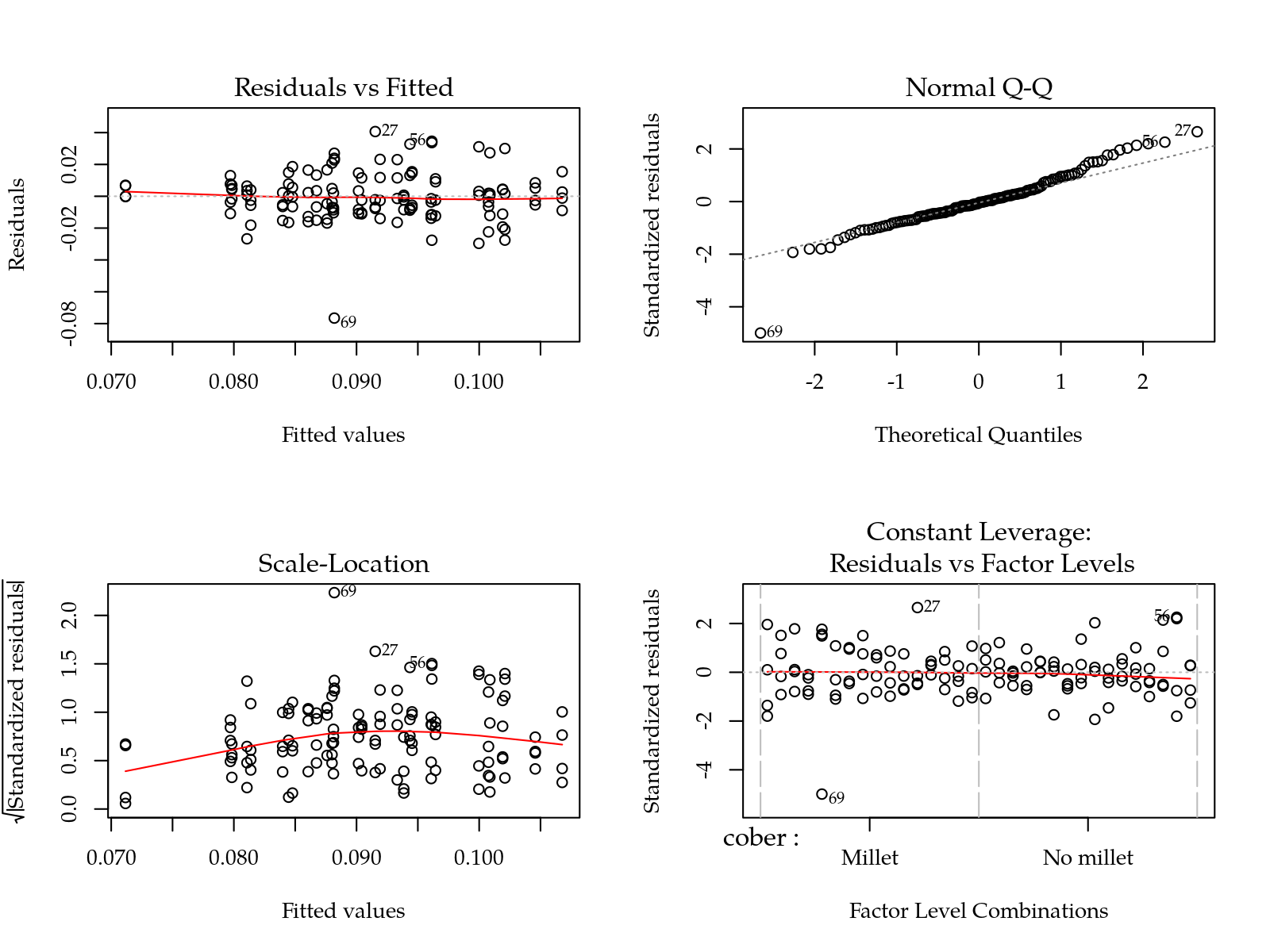
# MASS::boxcox(m0)

im <- influence.measures(m0)
# summary(im)

del <- im$is.inf[, "dffit"]
m0 <- update(m0, data = params[!del, ])
anova(m0)
## Analysis of Variance Table
##
## Response: Ur
## Df Sum Sq Mean Sq F value Pr(>F)
## cober 1 0.0000014 0.0000014 0.0065 0.93587
## gesso 1 0.0000746 0.0000746 0.3481 0.55642
## prof 1 0.0014229 0.0014229 6.6376 0.01134 *
## varie 3 0.0007300 0.0002433 1.1351 0.33826
## cober:gesso 1 0.0044550 0.0044550 20.7815 1.363e-05 ***
## cober:prof 1 0.0000297 0.0000297 0.1384 0.71056
## cober:varie 3 0.0015884 0.0005295 2.4699 0.06580 .
## gesso:prof 1 0.0002396 0.0002396 1.1176 0.29280
## gesso:varie 3 0.0002934 0.0000978 0.4563 0.71340
## prof:varie 3 0.0001364 0.0000455 0.2121 0.88785
## Residuals 108 0.0231522 0.0002144
## ---
## Signif. codes: 0 '***' 0.001 '**' 0.01 '*' 0.05 '.' 0.1 ' ' 1#-----------------------------------------------------------------------
# Desdobramento.
# Estimativas para as profundidades.
Xm <- LE_matrix(m0, effect = "prof")
rownames(Xm) <- levels(db$prof)
g1 <- apmc(X = Xm, model = m0, focus = "prof")
g1## prof fit lwr upr cld
## 1 0-0.05 0.09509044 0.09146270 0.09871818 a
## 2 0.05-0.20 0.08861510 0.08495424 0.09227597 b# Desdobrar gesso dentro de cobertura.
LSmeans(m0, effect = c("gesso", "cober"))## Coefficients:
## estimate se df t.stat p.value
## [1,] 9.7136e-02 2.6353e-03 1.0800e+02 3.6859e+01 0
## [2,] 8.6514e-02 2.5883e-03 1.0800e+02 3.3426e+01 0
## [3,] 8.5203e-02 2.5883e-03 1.0800e+02 3.2919e+01 0
## [4,] 9.8558e-02 2.5883e-03 1.0800e+02 3.8079e+01 0Xm <- LE_matrix(m0, effect = c("gesso", "cober"))
grid <- equallevels(attr(Xm, "grid"), db)
L <- by(Xm, INDICES = grid$cober, FUN = as.matrix)
L <- lapply(L, "rownames<-", levels(grid$gesso))
g2 <- lapply(L, apmc, model = m0, focus = "gesso")
g2## $Millet
## gesso fit lwr upr cld
## 1 0 0.09713565 0.09191197 0.10235934 b
## 2 4 0.08651437 0.08138398 0.09164477 a
##
## $`No millet`
## gesso fit lwr upr cld
## 1 0 0.08520292 0.08007252 0.09033331 b
## 2 4 0.09855814 0.09342775 0.10368854 ag2 <- ldply(g2)
names(g2)[1] <- "cober"
g2 <- equallevels(g2, db)#-----------------------------------------------------------------------
# Gráfico.
p1 <- segplot(prof ~ lwr + upr, centers = fit, data = g1, draw = FALSE,
xlab = expression("Residual moisture"~(m^3~m^{-3})),
ylab = "Soil layer (m)") +
layer(panel.text(x = centers, y = z, labels = g1$cld, pos = 3))
p2 <- segplot(cober ~ lwr + upr, centers = fit, data = g2, draw = FALSE,
groups = g2$gesso, pch = g2$gesso, gap = 0.1,
panel = panel.groups.segplot,
xlab = expression("Residual moisture"~(m^3~m^{-3})),
ylab = "Cover crop",
key = list(columns = 2, type = "o", divide = 1,
title = expression("Gypsum"~(ton~ha^{-1})),
cex.title = 1.1,
lines = list(pch = 1:2),
text = list(levels(g2$gesso)))) +
layer(panel.text(x = centers,
y = as.numeric(z) +
gap * (2 * ((as.numeric(groups) - 1)/
(nlevels(groups) - 1)) - 1),
labels = cld, pos = 3), data = g2)
p2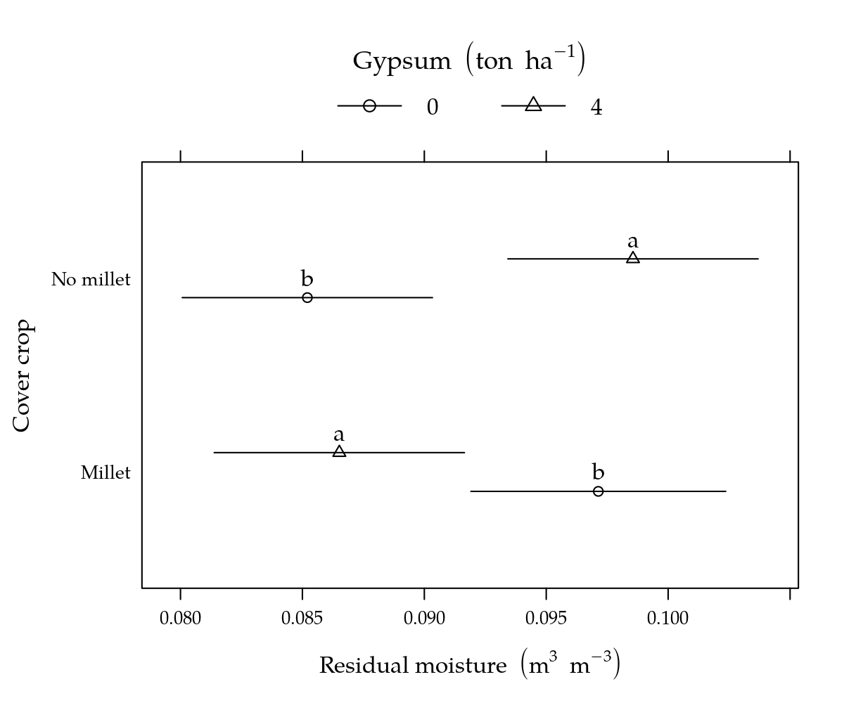
# x11(width = 6, height = 5)
d <- 0.6
plot(p1, position = c(0, d, 1, 1), more = TRUE)
plot(p2, position = c(0, 0, 1, d), more = FALSE)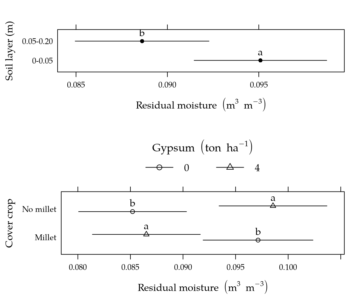
Us: umidade de saturação
#-----------------------------------------------------------------------
# Análise do Us.
m0 <- lm(Us ~ (cober + gesso + prof + varie)^2, data = params)
par(mfrow = c(2,2)); plot(m0); layout(1)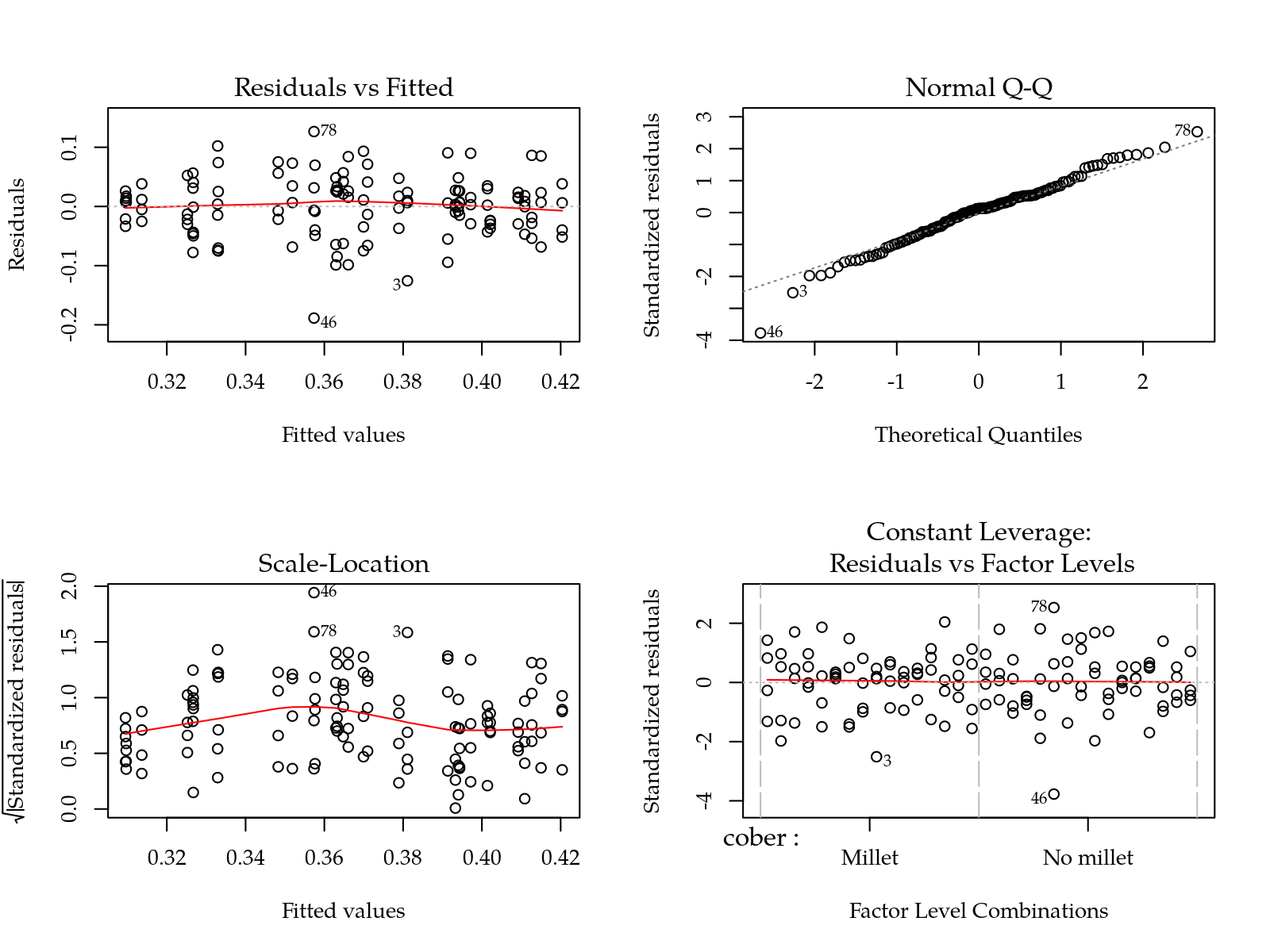
# MASS::boxcox(m0)
im <- influence.measures(m0)
# summary(im)
del <- im$is.inf[, "dffit"]
m0 <- update(m0, data = params[!del,])
anova(m0)## Analysis of Variance Table
##
## Response: Us
## Df Sum Sq Mean Sq F value Pr(>F)
## cober 1 0.004879 0.004879 1.8945 0.17154
## gesso 1 0.001788 0.001788 0.6943 0.40656
## prof 1 0.075827 0.075827 29.4400 3.566e-07 ***
## varie 3 0.001157 0.000386 0.1497 0.92967
## cober:gesso 1 0.006721 0.006721 2.6095 0.10914
## cober:prof 1 0.003100 0.003100 1.2037 0.27503
## cober:varie 3 0.009740 0.003247 1.2606 0.29165
## gesso:prof 1 0.003934 0.003934 1.5275 0.21916
## gesso:varie 3 0.003474 0.001158 0.4496 0.71806
## prof:varie 3 0.030415 0.010138 3.9362 0.01041 *
## Residuals 108 0.278168 0.002576
## ---
## Signif. codes: 0 '***' 0.001 '**' 0.01 '*' 0.05 '.' 0.1 ' ' 1#-----------------------------------------------------------------------
# Desdobramento.
# Desdobrar prof dentro de varie.
LSmeans(m0, effect = c("prof", "varie"))## Coefficients:
## estimate se df t.stat p.value
## [1,] 0.374267 0.012688 108.000000 29.498499 0
## [2,] 0.372329 0.012688 108.000000 29.345739 0
## [3,] 0.393543 0.012688 108.000000 31.017730 0
## [4,] 0.353244 0.013145 108.000000 26.872827 0
## [5,] 0.409894 0.012688 108.000000 32.306454 0
## [6,] 0.327029 0.012688 108.000000 25.775344 0
## [7,] 0.399921 0.012688 108.000000 31.520468 0
## [8,] 0.331721 0.012688 108.000000 26.145176 0Xm <- LE_matrix(m0, effect = c("prof", "varie"))
grid <- equallevels(attr(Xm, "grid"), db)
L <- by(Xm, INDICES = grid$varie, FUN = as.matrix)
L <- lapply(L, "rownames<-", levels(grid$prof))
g2 <- lapply(L, apmc, model = m0, focus = "prof")
g2## $`IAC Fantastico`
## prof fit lwr upr cld
## 1 0-0.05 0.3742672 0.3491181 0.3994164 a
## 2 0.05-0.20 0.3723291 0.3471799 0.3974782 a
##
## $Imperial
## prof fit lwr upr cld
## 1 0-0.05 0.3935427 0.3683936 0.4186919 a
## 2 0.05-0.20 0.3532441 0.3271884 0.3792998 b
##
## $Perola
## prof fit lwr upr cld
## 1 0-0.05 0.4098936 0.3847445 0.4350428 a
## 2 0.05-0.20 0.3270291 0.3018799 0.3521782 b
##
## $`Smooth cayenne`
## prof fit lwr upr cld
## 1 0-0.05 0.3999213 0.3747722 0.4250705 a
## 2 0.05-0.20 0.3317214 0.3065722 0.3568705 bg2 <- ldply(g2); names(g2)[1] <- "varie"
g2 <- equallevels(g2, db)#-----------------------------------------------------------------------
# Gráfico.
p2 <- segplot(varie ~ lwr + upr, centers = fit, data = g2, draw = FALSE,
groups = g2$prof, pch = g2$prof, gap = 0.1,
panel = panel.groups.segplot,
xlab = expression("Saturation moisture"~(m^3~m^{-3})),
ylab = expression(Gypsum~(ton~ha^{-1})),
key = list(columns = 2, type = "o", divide = 1,
title = "Soil layer (m)", cex.title = 1.1,
lines = list(pch = 1:2),
text = list(levels(g2$prof)))) +
layer(panel.text(x = centers,
y = as.numeric(z) +
gap * (2 * ((as.numeric(groups) - 1)/
(nlevels(groups) - 1)) - 1),
labels = cld, pos = 3), data = g2)
p2
alpha: parâmetro empírico da curva de retenção
#-----------------------------------------------------------------------
# Análise do alpha.
# min(params$alp)
# Para atender os pressupostos, somou-se 1.5 para não ter valores
# negativos e elevou-se ao quadrado.
m0 <- lm(c(alp + 1.5)^2 ~ (cober + gesso + prof + varie)^2,
data = params)
par(mfrow = c(2,2)); plot(m0); layout(1)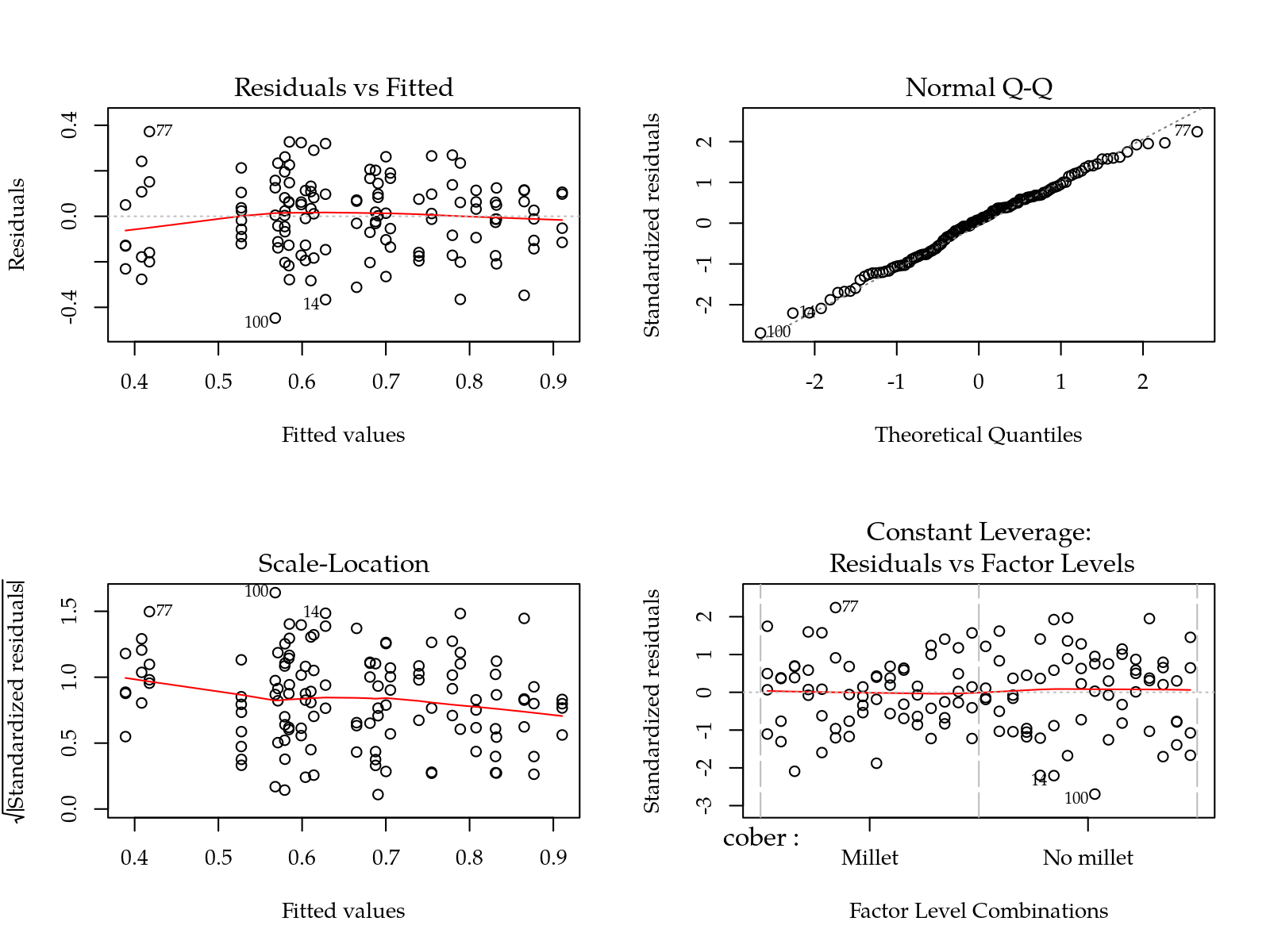
# MASS::boxcox(m0)
im <- influence.measures(m0)
# summary(im)
del <- im$is.inf[, "dffit"]
m0 <- update(m0, data = params[!del,])
anova(m0)## Analysis of Variance Table
##
## Response: c(alp + 1.5)^2
## Df Sum Sq Mean Sq F value Pr(>F)
## cober 1 0.0170 0.01700 0.5250 0.4702859
## gesso 1 0.0032 0.00319 0.0986 0.7541183
## prof 1 0.9220 0.92203 28.4690 5.222e-07 ***
## varie 3 0.0348 0.01161 0.3584 0.7831649
## cober:gesso 1 0.2338 0.23375 7.2174 0.0083508 **
## cober:prof 1 0.0018 0.00181 0.0559 0.8136096
## cober:varie 3 0.2634 0.08779 2.7107 0.0485873 *
## gesso:prof 1 0.0394 0.03940 1.2165 0.2724814
## gesso:varie 3 0.1655 0.05518 1.7038 0.1704988
## prof:varie 3 0.5929 0.19765 6.1026 0.0007069 ***
## Residuals 109 3.5302 0.03239
## ---
## Signif. codes: 0 '***' 0.001 '**' 0.01 '*' 0.05 '.' 0.1 ' ' 1# Como o alpha é um parâmetro empírico, de quase nenhum significado
# aplicado, não será feito o desdobramento da interação. As diferenças
# em alpha podem implicar em diferenças no parâmetro S que é mais
# interpretável. Abaixo segem as estimativas.
# Os valores abaixo são para simples conferência. Lembrar que estão na
# escala transformada y_t = (y + 1.5)^2.
LSmeans(m0, effect = c("prof", "varie"))## Coefficients:
## estimate se df t.stat p.value
## [1,] 0.633662 0.044991 109.000000 14.084141 0
## [2,] 0.692250 0.044991 109.000000 15.386358 0
## [3,] 0.750862 0.044991 109.000000 16.689099 0
## [4,] 0.556792 0.044991 109.000000 12.375594 0
## [5,] 0.828054 0.044991 109.000000 18.404808 0
## [6,] 0.539282 0.044991 109.000000 11.986398 0
## [7,] 0.765417 0.044991 109.000000 17.012593 0
## [8,] 0.510687 0.044991 109.000000 11.350829 0LSmeans(m0, effect = c("gesso", "cober"))## Coefficients:
## estimate se df t.stat p.value
## [1,] 0.633412 0.031814 109.000000 19.910121 0
## [2,] 0.708890 0.031814 109.000000 22.282633 0
## [3,] 0.695829 0.031814 109.000000 21.872096 0
## [4,] 0.600372 0.031814 109.000000 18.871576 0LSmeans(m0, effect = c("cober", "varie"))## Coefficients:
## estimate se df t.stat p.value
## [1,] 0.665049 0.044991 109.000000 14.781760 0
## [2,] 0.660864 0.044991 109.000000 14.688739 0
## [3,] 0.595163 0.044991 109.000000 13.228446 0
## [4,] 0.712491 0.044991 109.000000 15.836247 0
## [5,] 0.739759 0.044991 109.000000 16.442304 0
## [6,] 0.627577 0.044991 109.000000 13.948902 0
## [7,] 0.684633 0.044991 109.000000 15.217056 0
## [8,] 0.591470 0.044991 109.000000 13.146365 0n: parâmetro empírico da curva de retenção
#-----------------------------------------------------------------------
# Análise do n (na escala log para atender pressupostos).
m0 <- lm(log(n) ~ (cober + gesso + prof + varie)^2, data = params)
par(mfrow = c(2,2)); plot(m0); layout(1)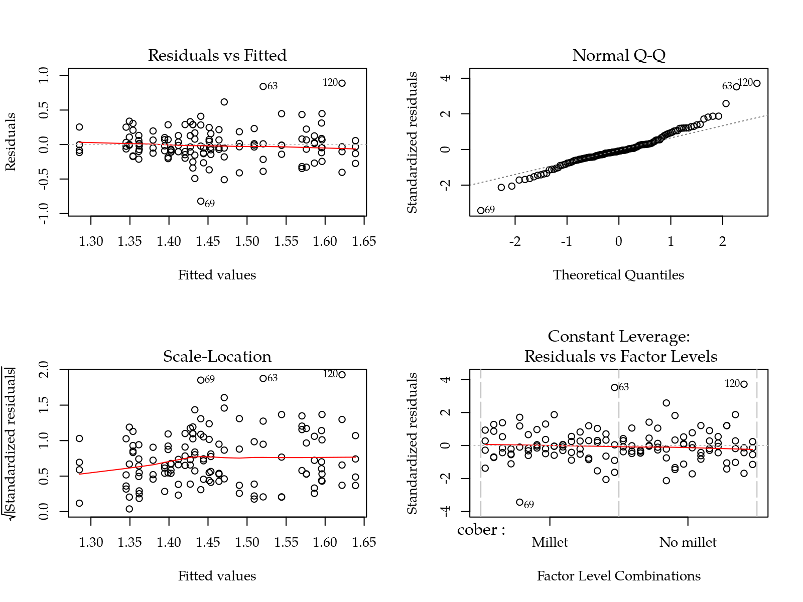
# MASS::boxcox(m0)
im <- influence.measures(m0)
# summary(im)
del <- im$is.inf[, "dffit"]
m0 <- update(m0, data = params[!del,])
anova(m0)## Analysis of Variance Table
##
## Response: log(n)
## Df Sum Sq Mean Sq F value Pr(>F)
## cober 1 0.0000 0.000044 0.0010 0.97504
## gesso 1 0.0185 0.018477 0.4112 0.52277
## prof 1 0.1573 0.157337 3.5010 0.06409 .
## varie 3 0.0586 0.019536 0.4347 0.72860
## cober:gesso 1 0.1855 0.185518 4.1281 0.04468 *
## cober:prof 1 0.0232 0.023209 0.5164 0.47394
## cober:varie 3 0.2020 0.067343 1.4985 0.21923
## gesso:prof 1 0.0864 0.086430 1.9232 0.16841
## gesso:varie 3 0.1008 0.033607 0.7478 0.52597
## prof:varie 3 0.1503 0.050088 1.1145 0.34661
## Residuals 106 4.7637 0.044941
## ---
## Signif. codes: 0 '***' 0.001 '**' 0.01 '*' 0.05 '.' 0.1 ' ' 1# Desdobramento não realizado por argumentos iguais aos do parâmetro
# alpha.
LSmeans(m0, effect = c("gesso", "cober"))## Coefficients:
## estimate se df t.stat p.value
## [1,] 1.505749 0.038157 106.000000 39.462205 0
## [2,] 1.400516 0.038157 106.000000 36.704289 0
## [3,] 1.425495 0.037475 106.000000 38.038346 0
## [4,] 1.476608 0.038157 106.000000 38.698497 0Parâmetro S: taxa da curva de retenção no ponto de inflexão
#-----------------------------------------------------------------------
# Parâmetro S: slope da curva de retenção no ponto de inflexão.
# Calcular o S a partir das estimativas dos parâmetros da CRA.
params$S <- with(params, {
m <- 1 - 1/n
d <- Us - Ur
-d * n * (1 + 1/m)^(-m - 1)
})
m0 <- lm(S ~ (cober + gesso + prof + varie)^2, data = params)
par(mfrow = c(2,2)); plot(m0); layout(1)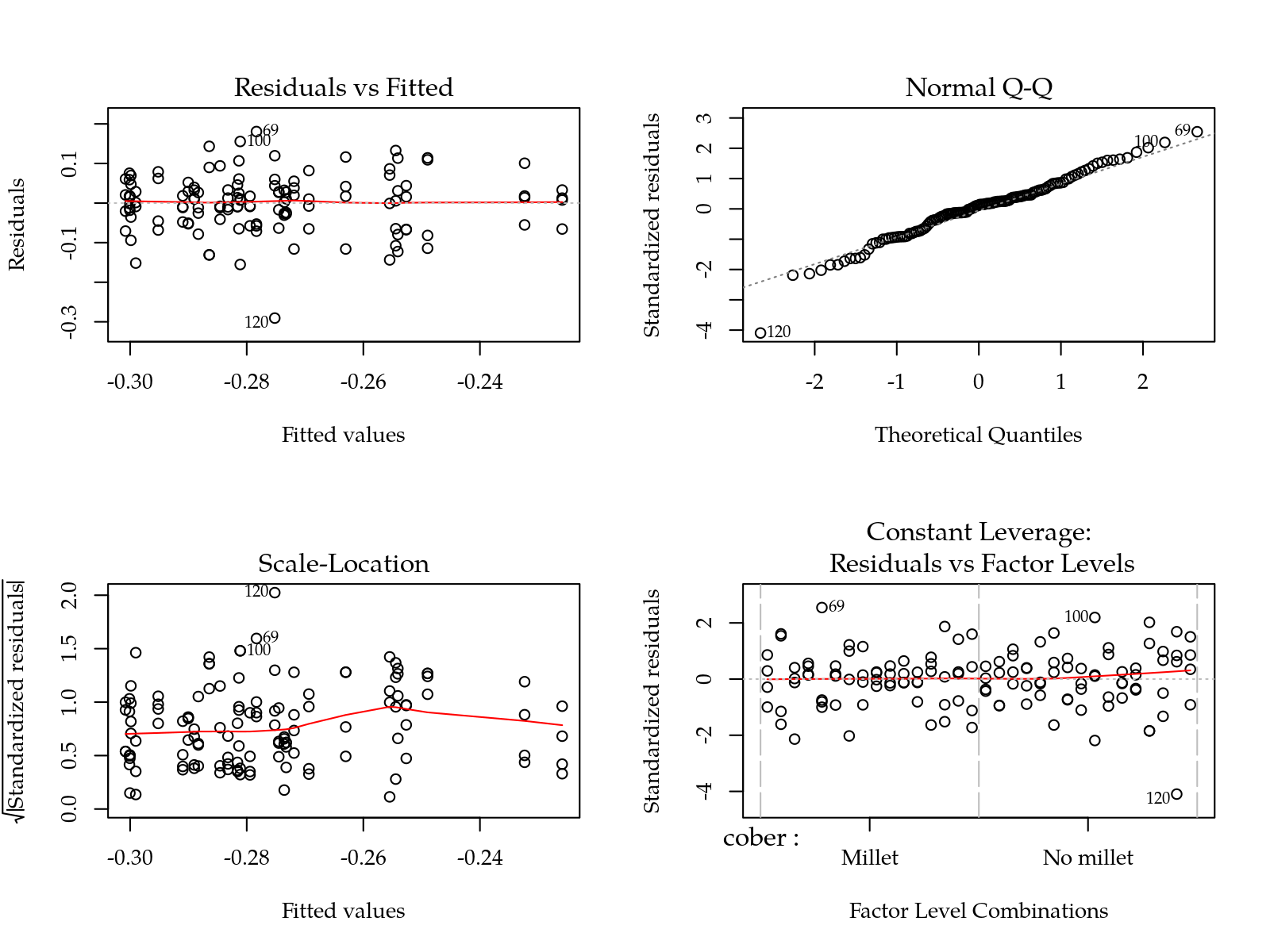
# MASS::boxcox(m0)
im <- influence.measures(m0)
# summary(im)
del <- im$is.inf[,"dffit"]
m0 <- update(m0, data = params[!del, ])
anova(m0)## Analysis of Variance Table
##
## Response: S
## Df Sum Sq Mean Sq F value Pr(>F)
## cober 1 0.00161 0.0016143 0.3199 0.5728
## gesso 1 0.00008 0.0000810 0.0160 0.8994
## prof 1 0.01025 0.0102480 2.0310 0.1570
## varie 3 0.00700 0.0023324 0.4622 0.7092
## cober:gesso 1 0.00001 0.0000115 0.0023 0.9621
## cober:prof 1 0.00463 0.0046337 0.9183 0.3401
## cober:varie 3 0.00400 0.0013327 0.2641 0.8511
## gesso:prof 1 0.00183 0.0018293 0.3625 0.5484
## gesso:varie 3 0.02074 0.0069133 1.3701 0.2558
## prof:varie 3 0.01092 0.0036408 0.7215 0.5412
## Residuals 108 0.54495 0.0050458# Não existe efeito dos fatores experimentais sobre o S.
LSmeans(m0)## Coefficients:
## estimate se df t.stat p.value
## estimate -0.2733963 0.0063073 108.0000000 -43.3460573 0I: tensão correspondente ao ponto de inflexão
#-----------------------------------------------------------------------
# Parâmetro I: tensão correspondente ao ponto de inflexão.
# Calcular o I a partir das estimativas dos parâmetros da CRA.
params$I <- with(params, {
m <- 1 - 1/n
-alp - log(m)/n
})
# Análise sobre o recíproco de I para atender os pressupostos.
m0 <- lm(1/I ~ (cober + gesso + prof + varie)^2, data = params)
par(mfrow = c(2,2)); plot(m0); layout(1)
# MASS::boxcox(m0)
im <- influence.measures(m0)
# summary(im)
del <- im$is.inf[, "dffit"]
m0 <- update(m0, data = params[!del, ])
anova(m0)## Analysis of Variance Table
##
## Response: 1/I
## Df Sum Sq Mean Sq F value Pr(>F)
## cober 1 0.0076 0.00764 0.2179 0.641552
## gesso 1 0.0014 0.00142 0.0406 0.840757
## prof 1 0.9900 0.99000 28.2402 5.735e-07 ***
## varie 3 0.0419 0.01396 0.3982 0.754568
## cober:gesso 1 0.1745 0.17452 4.9781 0.027716 *
## cober:prof 1 0.0202 0.02022 0.5768 0.449221
## cober:varie 3 0.2606 0.08687 2.4780 0.065085 .
## gesso:prof 1 0.0536 0.05364 1.5302 0.218736
## gesso:varie 3 0.1980 0.06601 1.8829 0.136728
## prof:varie 3 0.4783 0.15943 4.5477 0.004829 **
## Residuals 109 3.8211 0.03506
## ---
## Signif. codes: 0 '***' 0.001 '**' 0.01 '*' 0.05 '.' 0.1 ' ' 1#-----------------------------------------------------------------------
# Desdobramentos.
# Desdobrar prof dentro de varie.
LSmeans(m0, effect = c("prof", "varie"))## Coefficients:
## estimate se df t.stat p.value
## [1,] 1.319915 0.046808 109.000000 28.198265 0
## [2,] 1.339459 0.046808 109.000000 28.615790 0
## [3,] 1.415107 0.046808 109.000000 30.231911 0
## [4,] 1.238376 0.046808 109.000000 26.456294 0
## [5,] 1.520414 0.046808 109.000000 32.481662 0
## [6,] 1.210782 0.046808 109.000000 25.866775 0
## [7,] 1.436758 0.046808 109.000000 30.694454 0
## [8,] 1.200014 0.046808 109.000000 25.636734 0Xm <- LE_matrix(m0, effect = c("prof", "varie"))
grid <- equallevels(attr(Xm, "grid"), db)
L <- by(Xm, INDICES = grid$varie, FUN = as.matrix)
L <- lapply(L, "rownames<-", levels(grid$prof))
g1 <- lapply(L, apmc, model = m0, focus = "prof")
g1## $`IAC Fantastico`
## prof fit lwr upr cld
## 1 0-0.05 1.319915 1.227142 1.412688 a
## 2 0.05-0.20 1.339459 1.246686 1.432231 a
##
## $Imperial
## prof fit lwr upr cld
## 1 0-0.05 1.415107 1.322334 1.507879 a
## 2 0.05-0.20 1.238376 1.145603 1.331149 b
##
## $Perola
## prof fit lwr upr cld
## 1 0-0.05 1.520414 1.427641 1.613187 a
## 2 0.05-0.20 1.210782 1.118009 1.303554 b
##
## $`Smooth cayenne`
## prof fit lwr upr cld
## 1 0-0.05 1.436758 1.343985 1.529530 a
## 2 0.05-0.20 1.200014 1.107241 1.292787 bg1 <- ldply(g1); names(g1)[1] <- "varie"
g1 <- equallevels(g1, db)
g1[, c("fit","lwr","upr")] <- exp(1/g1[, c("fit","lwr","upr")])
# Desdobrar gesso dentro de cobertura.
LSmeans(m0, effect = c("gesso", "cober"))
## Coefficients:
## estimate se df t.stat p.value
## [1,] 1.309237 0.033099 109.000000 39.555770 0
## [2,] 1.376420 0.033099 109.000000 41.585540 0
## [3,] 1.367635 0.033099 109.000000 41.320115 0
## [4,] 1.287120 0.033099 109.000000 38.887533 0Xm <- LE_matrix(m0, effect = c("gesso", "cober"))
grid <- equallevels(attr(Xm, "grid"), db)
L <- by(Xm, INDICES = grid$cober, FUN = as.matrix)
L <- lapply(L, "rownames<-", levels(grid$gesso))
g3 <- lapply(L, apmc, model = m0, focus = "gesso")
g3## $Millet
## gesso fit lwr upr cld
## 1 0 1.309237 1.243637 1.374838 a
## 2 4 1.376420 1.310820 1.442020 a
##
## $`No millet`
## gesso fit lwr upr cld
## 1 0 1.367635 1.302034 1.433235 a
## 2 4 1.287120 1.221520 1.352720 ag3 <- ldply(g3); names(g3)[1] <- "cober"
g3 <- equallevels(g3, db)
g3[, c("fit","lwr","upr")] <- exp(1/g3[, c("fit","lwr","upr")])#-----------------------------------------------------------------------
# Gráfico.
p1 <- segplot(varie ~ lwr + upr, centers = fit, data = g1, draw = FALSE,
groups = g1$prof, pch = g1$prof, gap = 0.1,
panel = panel.groups.segplot,
# xlab = expression(log ~ da ~ tensão ~ (kPa)),
xlab = expression(Tension ~ (kPa)),
ylab = "Variety",
key = list(columns = 2, type = "o", divide = 1,
title = "Soil layer (m)", cex.title = 1.1,
lines = list(pch = 1:2),
text = list(levels(g1$prof)))) +
layer(panel.text(x = centers,
y = as.numeric(z) +
gap * (2 * ((as.numeric(groups) - 1)/
(nlevels(groups) - 1)) - 1),
labels = cld, pos = 3), data = g1)
p3 <- segplot(cober ~ lwr + upr, centers = fit, data = g3, draw = FALSE,
groups = g3$gesso, pch = g3$gesso, gap = 0.1,
panel = panel.groups.segplot,
# xlab = expression(log ~ da ~ tensão ~ (kPa)),
xlab = expression(Tension ~ (kPa)),
ylab = "Crop cover",
key = list(columns = 2, type = "o", divide = 1,
title = expression(Gypsum ~ (ton ~ ha^{-1})),
cex.title = 1.1,
lines = list(pch = 1:2),
text = list(levels(g3$gesso)))) +
layer(panel.text(x = centers,
y = as.numeric(z) +
gap * (2 * ((as.numeric(groups) - 1)/
(nlevels(groups) - 1)) - 1),
labels = cld, pos = 3), data = g3)
plot(p3, position = c(0, 0.6, 1, 1), more = TRUE)
plot(p1, position = c(0, 0, 1, 0.6), more = FALSE)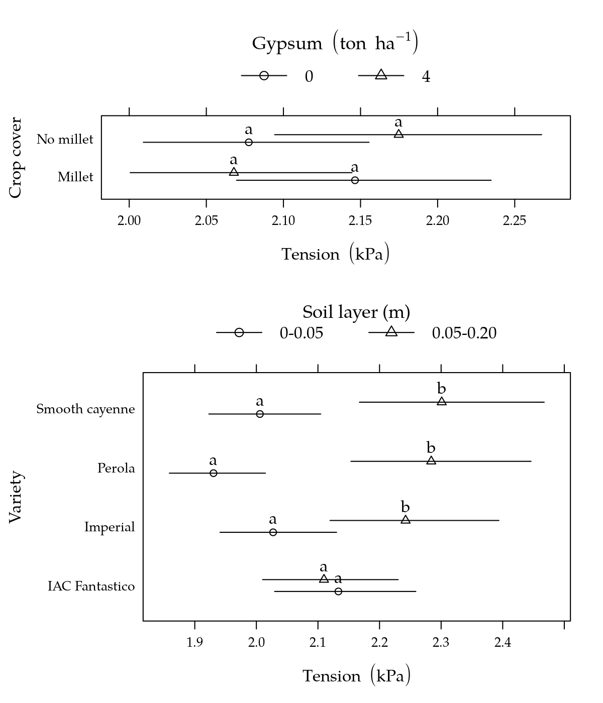
Parâmetro CAD: Capacidade de água disponível
#-----------------------------------------------------------------------
# Parâmetro CAD: Conteúdo de água disponível (CAD = UI-Ur).
# Calcular a umidade na tensão e a diferência de umidade com relação à
# residual.
params$UI <- with(params, {
UI <- Ur + (Us - Ur)/(1 + exp(n*(alp + I)))^(1 - 1/n)
UI - Ur
})
m0 <- lm(UI ~ (cober + gesso + prof + varie)^2, data = params)
par(mfrow = c(2,2)); plot(m0); layout(1)
# MASS::boxcox(m0)

im <- influence.measures(m0)
# summary(im)

del <- im$is.inf[, "dffit"]
m0 <- update(m0, data = params[!del,])
anova(m0)
## Analysis of Variance Table
##
## Response: UI
## Df Sum Sq Mean Sq F value Pr(>F)
## cober 1 0.000885 0.0008848 1.2490 0.266220
## gesso 1 0.000937 0.0009368 1.3225 0.252689
## prof 1 0.015630 0.0156296 22.0631 7.807e-06 ***
## varie 3 0.001306 0.0004352 0.6144 0.607131
## cober:gesso 1 0.005961 0.0059612 8.4150 0.004510 **
## cober:prof 1 0.000659 0.0006589 0.9301 0.336995
## cober:varie 3 0.002605 0.0008682 1.2256 0.304028
## gesso:prof 1 0.000801 0.0008011 1.1308 0.289966
## gesso:varie 3 0.000626 0.0002086 0.2945 0.829282
## prof:varie 3 0.011551 0.0038503 5.4351 0.001611 **
## Residuals 108 0.076507 0.0007084
## ---
## Signif. codes: 0 '***' 0.001 '**' 0.01 '*' 0.05 '.' 0.1 ' ' 1#--------------------------------------------
# Desdobramentos.
# Desdobrar prof dentro de varie.
LSmeans(m0, effect = c("prof", "varie"))## Coefficients:
## estimate se df t.stat p.value
## [1,] 1.4677e-01 6.6540e-03 1.0800e+02 2.2058e+01 0
## [2,] 1.5521e-01 6.6540e-03 1.0800e+02 2.3325e+01 0
## [3,] 1.6075e-01 6.6540e-03 1.0800e+02 2.4159e+01 0
## [4,] 1.4054e-01 6.8938e-03 1.0800e+02 2.0386e+01 0
## [5,] 1.6547e-01 6.6540e-03 1.0800e+02 2.4868e+01 0
## [6,] 1.2510e-01 6.6540e-03 1.0800e+02 1.8800e+01 0
## [7,] 1.6100e-01 6.6540e-03 1.0800e+02 2.4196e+01 0
## [8,] 1.2569e-01 6.6540e-03 1.0800e+02 1.8890e+01 0Xm <- LE_matrix(m0, effect = c("prof", "varie"))
grid <- equallevels(attr(Xm, "grid"), db)
L <- by(Xm, INDICES = grid$varie, FUN = as.matrix)
L <- lapply(L, "rownames<-", levels(grid$prof))
g1 <- lapply(L, apmc, model = m0, focus = "prof")
g1## $`IAC Fantastico`
## prof fit lwr upr cld
## 1 0-0.05 0.1467745 0.1335852 0.1599638 a
## 2 0.05-0.20 0.1552068 0.1420175 0.1683961 a
##
## $Imperial
## prof fit lwr upr cld
## 1 0-0.05 0.1607525 0.1475632 0.1739418 a
## 2 0.05-0.20 0.1405351 0.1268704 0.1541998 b
##
## $Perola
## prof fit lwr upr cld
## 1 0-0.05 0.1654711 0.1522818 0.1786603 a
## 2 0.05-0.20 0.1250955 0.1119062 0.1382848 b
##
## $`Smooth cayenne`
## prof fit lwr upr cld
## 1 0-0.05 0.1609968 0.1478075 0.1741861 a
## 2 0.05-0.20 0.1256906 0.1125013 0.1388799 bg1 <- ldply(g1)
names(g1)[1] <- "varie"
g1 <- equallevels(g1, db)
# Desdobrar gesso dentro de cobertura.
LSmeans(m0, effect = c("gesso", "cober"))## Coefficients:
## estimate se df t.stat p.value
## [1,] 1.4068e-01 4.7051e-03 1.0800e+02 2.9901e+01 0
## [2,] 1.4898e-01 4.7051e-03 1.0800e+02 3.1664e+01 0
## [3,] 1.6002e-01 4.7906e-03 1.0800e+02 3.3404e+01 0
## [4,] 1.4057e-01 4.7051e-03 1.0800e+02 2.9877e+01 0Xm <- LE_matrix(m0, effect = c("gesso", "cober"))
grid <- equallevels(attr(Xm, "grid"), db)
L <- by(Xm, INDICES = grid$cober, FUN = as.matrix)
L <- lapply(L, "rownames<-", levels(grid$gesso))
g3 <- lapply(L, apmc, model = m0, focus = "gesso")
g3## $Millet
## gesso fit lwr upr cld
## 1 0 0.1406845 0.1313582 0.1500107 a
## 2 4 0.1489789 0.1396527 0.1583052 a
##
## $`No millet`
## gesso fit lwr upr cld
## 1 0 0.1600236 0.1505278 0.1695194 a
## 2 4 0.1405744 0.1312481 0.1499006 bg3 <- ldply(g3)
names(g3)[1] <- "cober"
g3 <- equallevels(g3, db)#-----------------------------------------------------------------------
# Gráfico.
p1 <- segplot(varie ~ lwr + upr, centers = fit, data = g1, draw = FALSE,
groups = g1$prof, pch = g1$prof, gap = 0.1,
panel = panel.groups.segplot,
xlab = expression(
"Available water content"~ (m^3~m^{-3})),
ylab = "Variety",
key = list(columns = 2, type = "o", divide = 1,
title = "Soil layer (m)", cex.title = 1.1,
lines = list(pch = 1:2),
text = list(levels(g1$prof)))) +
layer(panel.text(x = centers,
y = as.numeric(z) +
gap * (2 * ((as.numeric(groups) - 1)/
(nlevels(groups) - 1)) - 1),
labels = cld, pos = 3), data = g1)
p3 <- segplot(cober ~ lwr + upr, centers = fit, data = g3, draw = FALSE,
groups = g3$gesso, pch = g3$gesso, gap = 0.1,
panel = panel.groups.segplot,
xlab = expression(
"Available water content" ~ (m^3 ~ m^{-3})),
ylab = "Crop cover",
key = list(columns = 2, type = "o", divide = 1,
title = expression(Gypsum ~ (ton ~ ha^{-1})),
cex.title = 1.1,
lines = list(pch = 1:2),
text = list(levels(g3$gesso)))) +
layer(panel.text(x = centers,
y = as.numeric(z) +
gap * (2 * ((as.numeric(groups) - 1)/
(nlevels(groups) - 1)) - 1),
labels = cld, pos = 3), data = g3)
plot(p3, position = c(0, 0.6, 1, 1), more = TRUE)
plot(p1, position = c(0, 0, 1, 0.6), more = FALSE)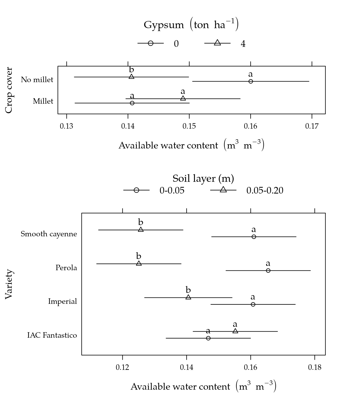
Informações da sessão
## quinta, 11 de julho de 2019, 20:05
## ----------------------------------------
## R version 3.6.1 (2019-07-05)
## Platform: x86_64-pc-linux-gnu (64-bit)
## Running under: Ubuntu 18.04.2 LTS
##
## Matrix products: default
## BLAS:   /usr/lib/x86_64-linux-gnu/blas/libblas.so.3.7.1
## LAPACK: /usr/lib/x86_64-linux-gnu/lapack/liblapack.so.3.7.1
##
## locale:
##  [1] LC_CTYPE=pt_BR.UTF-8       LC_NUMERIC=C
##  [3] LC_TIME=pt_BR.UTF-8        LC_COLLATE=en_US.UTF-8
##  [5] LC_MONETARY=pt_BR.UTF-8    LC_MESSAGES=en_US.UTF-8
##  [7] LC_PAPER=pt_BR.UTF-8       LC_NAME=C
##  [9] LC_ADDRESS=C               LC_TELEPHONE=C
## [11] LC_MEASUREMENT=pt_BR.UTF-8 LC_IDENTIFICATION=C
##
## attached base packages:
## [1] stats     graphics  grDevices utils     datasets  methods
## [7] base
##
## other attached packages:
##  [1] captioner_2.2.3     knitr_1.23          RDASC_0.0-6
##  [4] multcomp_1.4-10     TH.data_1.0-10      MASS_7.3-51.4
##  [7] survival_2.44-1.1   mvtnorm_1.0-11      doBy_4.6-2
## [10] plyr_1.8.4          reshape_0.8.8       nlme_3.1-140
## [13] latticeExtra_0.6-28 RColorBrewer_1.1-2  lattice_0.20-38
## [16] wzRfun_0.81
##
## loaded via a namespace (and not attached):
##  [1] Rcpp_1.0.1       compiler_3.6.1   pillar_1.4.2
##  [4] tools_3.6.1      digest_0.6.20    evaluate_0.14
##  [7] memoise_1.1.0    tibble_2.1.3     pkgconfig_2.0.2
## [10] rlang_0.4.0      Matrix_1.2-17    commonmark_1.7
## [13] rpanel_1.1-4     yaml_2.2.0       pkgdown_1.3.0
## [16] xfun_0.8         stringr_1.4.0    dplyr_0.8.3
## [19] roxygen2_6.1.1   xml2_1.2.0       desc_1.2.0
## [22] fs_1.3.1         rprojroot_1.3-2  grid_3.6.1
## [25] tidyselect_0.2.5 glue_1.3.1       R6_2.4.0
## [28] tcltk_3.6.1      rmarkdown_1.13   purrr_0.3.2
## [31] magrittr_1.5     codetools_0.2-16 splines_3.6.1
## [34] backports_1.1.4  htmltools_0.3.6  assertthat_0.2.1
## [37] sandwich_2.5-1   stringi_1.4.3    crayon_1.3.4
## [40] zoo_1.8-6