Efeito de Inseticidas no Parasitismo de Trichogramma em Ovos de Lagartas da Soja
Tamara Akemi Takahashi & Walmes Zeviani
2019-07-11
egg_parasitoid.RmdDefinições da Sessão
#-----------------------------------------------------------------------
# Carregando pacotes e funções necessárias.

# https://github.com/walmes/wzRfun
# devtools::install_github("walmes/wzRfun")
# devtools::load_all("~/repos/wzRfun")
library(wzRfun)
library(lattice)
library(latticeExtra)
library(plyr)
library(doBy)
library(multcomp)library(RDASC)Análise Exploratória
Estes dados são resultados de um experimento fatorial triplo, conduzido em laboratório, que estudou o efeito de 7 inseticidas no processo de pré parasitismo de duas espécies de Trichogramma em duas espécies de lagastas da soja (hospedeiros). Várias variáveis resposta foram registradas com a finalidade de descrever o efeito dos inseticidas para as espécies de parasitóide e hospedeiro, considerando por exemplo, o tempo de vida da fêmea ovopositora, o tempo para eclosão dos ovos, a razão sexual observada e a taxa de emergência dos ovos parasitados.
#-----------------------------------------------------------------------
# Estrutura dos dados.

str(egg_parasitoid)
## 'data.frame': 560 obs. of 12 variables:
## $ inset: Factor w/ 7 levels "Clorpirifós",..: 7 7 7 7 7 7 7 7 7 7 ...
## $ paras: Factor w/ 2 levels "Trichogramma atopovirilia",..: 1 1 1 1 1 1 1 1 1 1 ...
## $ hosp : Factor w/ 2 levels "Anticarsia gemmatalis",..: 1 1 1 1 1 1 1 1 1 1 ...
## $ rept : int 1 2 3 4 5 6 7 8 9 10 ...
## $ otot : int 10 10 10 10 10 10 10 10 10 10 ...
## $ mort : int 0 0 0 0 0 0 0 0 0 0 ...
## $ incub: int 8 8 9 8 8 8 8 8 8 8 ...
## $ opar : int 9 9 7 7 10 10 10 7 10 9 ...
## $ oeme : int 9 9 7 7 10 10 10 7 10 9 ...
## $ pne : int 0 0 0 0 0 0 0 0 0 0 ...
## $ macho: int 6 13 4 9 6 6 24 4 6 11 ...
## $ femea: int 15 4 8 5 15 25 0 15 18 9 ...# levels(egg_parasitoid$inset)
# Português Inglês
# Clorpirifós Chlorpyrifos
# Deltametrina Deltamethrin
# Espinetoram Spinetoram
# Flubendiamida Flubendiamide
# Indoxacarbe Indoxacarb
# Novalurom Novaluron
# Testemunha Control
l <- c("Chlorpyrifos",
"Deltamethrin",
"Spinetoram",
"Flubendiamide",
"Indoxacarb",
"Novaluron",
"Control")
# Níveis dos fatores experimentais.
summary(egg_parasitoid[, 1:3])## inset paras
## Clorpirifós :80 Trichogramma atopovirilia:280
## Deltametrina :80 Trichogramma pretiosum :280
## Espinetoram :80
## Flubendiamida :80
## Indoxacarbe :80
## Novalurom :80
## Testemunha :80
## hosp
## Anticarsia gemmatalis :280
## Chrysodeixis includens:280
##
##
##
##
## # Usando nomes curtos para os níveis.
egg <- egg_parasitoid
levels(egg$inset) <- substr(l, 0, 5)
levels(egg$paras) <- c("Atopo", "Preti")
levels(egg$hosp) <- c("Anti", "Chry")
# Letra maiúscula para representar os fatores estudados.
names(egg)[1:3] <- c("I", "P", "H")
# Tabela de frequencia planejada do experimento (7 x 2 x 2 com 20 rep.).
ftable(xtabs(~I + P + H, data = egg))## H Anti Chry
## I P
## Chlor Atopo 20 20
## Preti 20 20
## Delta Atopo 20 20
## Preti 20 20
## Spine Atopo 20 20
## Preti 20 20
## Flube Atopo 20 20
## Preti 20 20
## Indox Atopo 20 20
## Preti 20 20
## Noval Atopo 20 20
## Preti 20 20
## Contr Atopo 20 20
## Preti 20 20## H Anti Chry
## I P
## Chlor Atopo 0 0
## Preti 19 6
## Delta Atopo 18 3
## Preti 19 14
## Spine Atopo 9 5
## Preti 16 4
## Flube Atopo 20 19
## Preti 19 19
## Indox Atopo 20 18
## Preti 19 20
## Noval Atopo 20 20
## Preti 20 20
## Contr Atopo 20 20
## Preti 20 20Sobreviência da Fêmea
A sobreviência da fêmea, 24 horas após a liberação no tubo de ensaio para parasitar os ovos, é representada por uma variável (mort) dicotômica onde 1 indica que a fêmea sobreviveu e 0 que não não sobreviveu. A variável vivo é o oposto da variável mort.
# Desfechos de vivo: 1 = sobreviveu, 0 = não sobreviveu.
egg$vivo <- 1 - egg$mort
ftable(xtabs(vivo ~ I + P + H, data = egg))
## H Anti Chry
## I P
## Chlor Atopo 0 0
## Preti 10 7
## Delta Atopo 17 17
## Preti 20 18
## Spine Atopo 0 0
## Preti 3 2
## Flube Atopo 19 19
## Preti 19 19
## Indox Atopo 17 16
## Preti 19 20
## Noval Atopo 20 15
## Preti 20 20
## Contr Atopo 19 20
## Preti 20 20# Modelo saturado.
m0 <- glm(vivo ~ (I + P + H)^3,
data = subset(egg),
family = quasibinomial)
anova(m0, test = "F")## Analysis of Deviance Table
##
## Model: quasibinomial, link: logit
##
## Response: vivo
##
## Terms added sequentially (first to last)
##
##
## Df Deviance Resid. Df Resid. Dev F Pr(>F)
## NULL 559 677.25
## I 6 373.14 553 304.11 103.3906 < 2.2e-16 ***
## P 1 38.94 552 265.17 64.7455 5.587e-15 ***
## H 1 2.63 551 262.54 4.3720 0.037008 *
## I:P 6 13.16 545 249.38 3.6472 0.001476 **
## I:H 6 8.07 539 241.30 2.2369 0.038446 *
## P:H 1 0.07 538 241.23 0.1149 0.734816
## I:P:H 6 3.82 532 237.42 1.0578 0.386964
## ---
## Signif. codes: 0 '***' 0.001 '**' 0.01 '*' 0.05 '.' 0.1 ' ' 1## Analysis of Deviance Table
##
## Model: quasibinomial, link: logit
##
## Response: vivo
##
## Terms added sequentially (first to last)
##
##
## Df Deviance Resid. Df Resid. Dev F Pr(>F)
## NULL 559 677.25
## I 6 373.14 553 304.11 94.6738 < 2.2e-16 ***
## P 1 38.94 552 265.17 59.2868 6.561e-14 ***
## H 1 2.63 551 262.54 4.0034 0.045910 *
## I:P 6 13.16 545 249.38 3.3397 0.003071 **
## I:H 6 8.07 539 241.30 2.0483 0.057719 .
## ---
## Signif. codes: 0 '***' 0.001 '**' 0.01 '*' 0.05 '.' 0.1 ' ' 1anova(m1, m0, test = "F")## Analysis of Deviance Table
##
## Model 1: vivo ~ I + P + H + I:P + I:H
## Model 2: vivo ~ (I + P + H)^3
## Resid. Df Resid. Dev Df Deviance F Pr(>F)
## 1 539 241.30
## 2 532 237.42 7 3.8866 0.9231 0.488#-----------------------------------------------------------------------
# Comparações múltiplas.
lsm <- LE_matrix(m1, effect = c("I", "P", "H"))
grid <- equallevels(attr(lsm, "grid"), egg)
comp <- vector(mode = "list", length = 2)
# Hospedeiros dentro de inseticida x parasitóide.
L <- by(lsm, INDICES = with(grid, interaction(I, P)), FUN = as.matrix)
L <- lapply(L, "rownames<-", levels(egg$H))
cmp <- lapply(L, apmc, model = m1, focus = "H", cld2 = TRUE)
pred <- ldply(cmp)
cmp <- ldply(strsplit(pred$.id, "\\."))
pred <- cbind(as.data.frame(cmp), pred[, -1])
names(pred)[1:2] <- names(grid)[1:2]
names(pred)[ncol(pred)] <- "cldH"
comp[[1]] <- pred
# Inseticidas dentro de parasitóide e hospedeiro.
L <- by(lsm, INDICES = with(grid, interaction(H, P)), FUN = as.matrix)
L <- lapply(L, "rownames<-", levels(egg$I))
cmp <- lapply(L, apmc, model = m1, focus = "I", test = "fdr",
cld2 = TRUE)
pred <- ldply(cmp)
cmp <- ldply(strsplit(pred$.id, "\\."))
pred <- cbind(as.data.frame(cmp), pred[, -1])
# names(pred)[1:2] <- names(grid)[1:2]
names(pred)[1:2] <- c("H", "P")
names(pred)[ncol(pred)] <- "cldI"
pred[, ncol(pred)] <- toupper(pred[, ncol(pred)])
comp[[2]] <- pred
str(comp)## List of 2
## $ :'data.frame': 28 obs. of 7 variables:
## ..$ I : chr [1:28] "Chlor" "Chlor" "Delta" "Delta" ...
## ..$ P : chr [1:28] "Atopo" "Atopo" "Atopo" "Atopo" ...
## ..$ H : Factor w/ 2 levels "Anti","Chry": 1 2 1 2 1 2 1 2 1 2 ...
## ..$ fit : num [1:28] -20.29 -20.91 2.06 1.47 -20.35 ...
## ..$ lwr : num [1:28] -4438.185 -4438.804 1.03 0.611 -4457.432 ...
## ..$ upr : num [1:28] 4397.61 4396.99 3.08 2.33 4416.72 ...
## ..$ cldH: chr [1:28] "a" "a" "a" "a" ...
## $ :'data.frame': 28 obs. of 7 variables:
## ..$ H : chr [1:28] "Anti" "Anti" "Anti" "Anti" ...
## ..$ P : chr [1:28] "Atopo" "Atopo" "Atopo" "Atopo" ...
## ..$ I : Factor w/ 7 levels "Chlor","Contr",..: 1 3 7 4 5 6 2 1 3 7 ...
## ..$ fit : num [1:28] -20.29 2.06 -20.35 2.94 1.55 ...
## ..$ lwr : num [1:28] -4438.18 1.03 -4457.43 1.53 0.65 ...
## ..$ upr : num [1:28] 4397.61 3.08 4416.72 4.36 2.45 ...
## ..$ cldI: chr [1:28] "A" "A" "A" "A" ...pred <- merge(comp[[1]],
comp[[2]],
by = intersect(names(comp[[1]]), names(comp[[2]])))
#-----------------------------------------------------------------------
# Passa para a escala de probabilidade.
i <- c("fit", "lwr", "upr")
pred[, i] <- sapply(pred[, i], m1$family$linkinv)
# Ordena da tabela.
pred <- pred[with(pred, order(P, I, H)), ]
# Intervalos de confiança do tamanho do suporte terão apenas o ponto
# representado.
i <- pred$upr - pred$lwr > 0.99
if (any(i)) {
pred[i, ]$lwr <- pred[i, ]$lwr <- NA
}
# Reordena os níveis pela probalidade de sobreviência.
pred$I <- reorder(pred$I, pred$fit)
# Legenda.
key <- list(points = list(pch = c(1, 19)),
text = list(levels(egg_parasitoid$hosp), font = 3),
title = "Hosts", cex.title = 1.1)
pred$cld <- with(pred, paste(cldI, cldH, sep = ""))cap <-
"Estimated probability of surviving at 24h for each inseticide on two parasiods and two hosts. Segment is a confidence interval for the probability of surviving. Parasitoids estimates followed by the same lower letters in a insetice and host combination are not different at 5%. Inseticides estimates followed by the same lower letters in a parasitoid and host combination are not different at 5%."
cap <- fgn_("surv", cap)
pred$vjust <- -0.5
pred$vjust[pred$cld == "ABa"] <- 1.5
# Gráfico de segmentos.
segplot(I ~ lwr + upr | P,
centers = fit,
data = pred,
xlab = "Insecticides",
ylab = "Probability of surviving a 24h period",
draw = FALSE,
horizontal = FALSE,
groups = H,
key = key,
strip = strip.custom(
factor.levels = levels(egg_parasitoid$paras),
par.strip.text = list(font = 3)),
gap = 0.15,
cld = pred$cld,
panel = panel.groups.segplot,
pch = key$points$pch[as.integer(pred$H)]) +
layer({
a <- cld[which.max(nchar(cld))]
l <- cld[subscripts]
v <- pred$vjust[subscripts]
x <- as.integer(z)[subscripts] + centfac(groups[subscripts], gap)
y <- centers[subscripts]
# Usa símbolo unicode:
# http://www.alanwood.net/unicode/geometric_shapes.html
grid.text("\u25AE",
x = unit(x, "native"),
y = unit(y, "native"),
vjust = v,
gp = gpar(col = "white")
)
grid.text(l,
x = unit(x, "native"),
y = unit(y, "native"),
vjust = v,
gp = gpar(col = "black", fontsize = 10))
})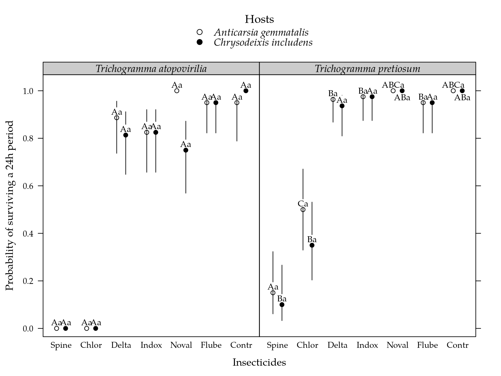
Figura 1: Estimated probability of surviving at 24h for each inseticide on two parasiods and two hosts. Segment is a confidence interval for the probability of surviving. Parasitoids estimates followed by the same lower letters in a insetice and host combination are not different at 5%. Inseticides estimates followed by the same lower letters in a parasitoid and host combination are not different at 5%.
Ovos Parasitados
#-----------------------------------------------------------------------
# Análise exploratória.

useOuterStrips(xyplot(opar/otot ~ I | H + P,
                      data = egg,
                      jitter.x = TRUE,
                      type = c("p", "a")))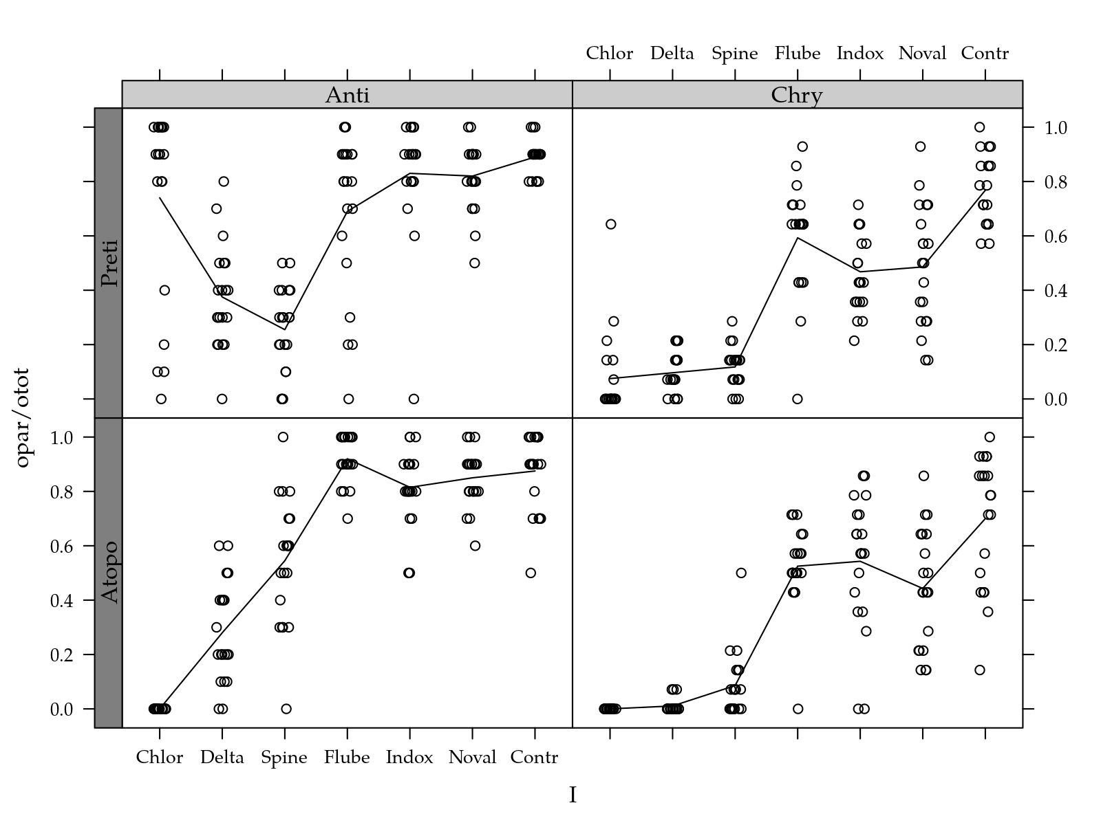
#-----------------------------------------------------------------------
# Ajuste do modelo.

m0 <- glm(cbind(opar, otot - opar) ~ I * P * H,
          data = egg,
          family = quasibinomial)

par(mfrow = c(2, 2))
plot(m0)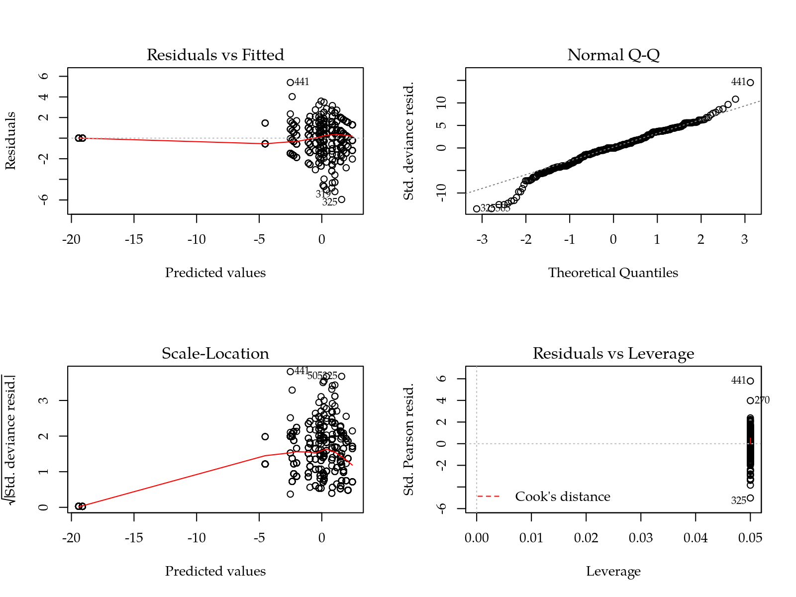
## Analysis of Deviance Table
##
## Model: quasibinomial, link: logit
##
## Response: cbind(opar, otot - opar)
##
## Terms added sequentially (first to last)
##
##
##       Df Deviance Resid. Df Resid. Dev        F    Pr(>F)
## NULL                    559     4142.3
## I      6  1768.10       553     2374.2 144.3558 < 2.2e-16 ***
## P      1    16.93       552     2357.3   8.2919 0.0041425 **
## H      1   736.09       551     1621.2 360.5869 < 2.2e-16 ***
## I:P    6   313.33       545     1307.9  25.5817 < 2.2e-16 ***
## I:H    6    87.99       539     1219.9   7.1843 2.202e-07 ***
## P:H    1    31.31       538     1188.6  15.3395 0.0001015 ***
## I:P:H  6    38.77       532     1149.8   3.1654 0.0046431 **
## ---
## Signif. codes:  0 '***' 0.001 '**' 0.01 '*' 0.05 '.' 0.1 ' ' 1
# summary(m0)
#-----------------------------------------------------------------------
# Comparações múltiplas.
lsm <- LE_matrix(m0, effect = c("I", "P", "H"))
grid <- equallevels(attr(lsm, "grid"), egg)
comp <- vector(mode = "list", length = 2)
# Hospedeiros dentro de inseticida x parasitóide.
L <- by(lsm, INDICES = with(grid, interaction(I, P)), FUN = as.matrix)
L <- lapply(L, "rownames<-", levels(egg$H))
cmp <- lapply(L, apmc, model = m0, focus = "H", cld2 = TRUE)
pred <- ldply(cmp)
cmp <- ldply(strsplit(pred$.id, "\\."))
pred <- cbind(as.data.frame(cmp), pred[, -1])
names(pred)[1:2] <- names(grid)[1:2]
names(pred)[ncol(pred)] <- "cldH"
comp[[1]] <- pred
# Inseticidas dentro de parasitóide e hospedeiro.
L <- by(lsm, INDICES = with(grid, interaction(H, P)), FUN = as.matrix)
L <- lapply(L, "rownames<-", levels(egg$I))
cmp <- lapply(L, apmc, model = m0, focus = "I", test = "fdr",
cld2 = TRUE)
pred <- ldply(cmp)
cmp <- ldply(strsplit(pred$.id, "\\."))
pred <- cbind(as.data.frame(cmp), pred[, -1])
# names(pred)[1:2] <- names(grid)[1:2]
names(pred)[1:2] <- c("H", "P")
names(pred)[ncol(pred)] <- "cldI"
pred[, ncol(pred)] <- toupper(pred[, ncol(pred)])
comp[[2]] <- pred
str(comp)## List of 2
## $ :'data.frame': 28 obs. of 7 variables:
## ..$ I : chr [1:28] "Chlor" "Chlor" "Delta" "Delta" ...
## ..$ P : chr [1:28] "Atopo" "Atopo" "Atopo" "Atopo" ...
## ..$ H : Factor w/ 2 levels "Anti","Chry": 1 2 1 2 1 2 1 2 1 2 ...
## ..$ fit : num [1:28] -19.118 -19.421 -0.944 -4.525 0.18 ...
## ..$ lwr : num [1:28] -1721.472 -1693.258 -1.385 -6.151 -0.217 ...
## ..$ upr : num [1:28] 1683.235 1654.416 -0.503 -2.9 0.578 ...
## ..$ cldH: chr [1:28] "a" "a" "b" "a" ...
## $ :'data.frame': 28 obs. of 7 variables:
## ..$ H : chr [1:28] "Anti" "Anti" "Anti" "Anti" ...
## ..$ P : chr [1:28] "Atopo" "Atopo" "Atopo" "Atopo" ...
## ..$ I : Factor w/ 7 levels "Chlor","Contr",..: 1 3 7 4 5 6 2 1 3 7 ...
## ..$ fit : num [1:28] -19.118 -0.944 0.18 2.442 1.483 ...
## ..$ lwr : num [1:28] -1721.472 -1.385 -0.217 1.712 0.973 ...
## ..$ upr : num [1:28] 1683.235 -0.503 0.578 3.172 1.993 ...
## ..$ cldI: chr [1:28] "ABC" "A" "B" "C" ...pred <- merge(comp[[1]],
comp[[2]],
by = intersect(names(comp[[1]]), names(comp[[2]])))
#-----------------------------------------------------------------------
# Passa para a escala de probabilidade.
i <- c("fit", "lwr", "upr")
pred[, i] <- sapply(pred[, i], m1$family$linkinv)
# Ordena da tabela.
pred <- pred[with(pred, order(P, I, H)), ]
# Intervalos de confiança do tamanho do suporte terão apenas o ponto
# representado.
i <- pred$upr - pred$lwr > 0.99
if (any(i)) {
pred[i, ]$lwr <- pred[i, ]$lwr <- NA
}
# Reordena os níveis pela probalidade de sobreviência.
pred$I <- reorder(pred$I, pred$fit)
# Legenda.
key <- list(points = list(pch = c(1, 19)),
text = list(levels(egg_parasitoid$hosp), font = 3),
title = "Hosts", cex.title = 1.1)
pred$cld <- with(pred, paste(cldI, cldH, sep = ""))
#-----------------------------------------------------------------------
ab <- aggregate(cbind(paras = opar/otot) ~ I + H + P,
data = egg,
FUN = mean)
kable(merge(pred, ab, by = intersect(names(pred), names(ab)))[, -c(5:9)])| I | P | H | fit | paras |
|---|---|---|---|---|
| Chlor | Atopo | Anti | 0.0000000 | 0.0000000 |
| Chlor | Atopo | Chry | 0.0000000 | 0.0000000 |
| Chlor | Preti | Anti | 0.7400000 | 0.7400000 |
| Chlor | Preti | Chry | 0.0750000 | 0.0750000 |
| Contr | Atopo | Anti | 0.8750000 | 0.8750000 |
| Contr | Atopo | Chry | 0.7000000 | 0.7000000 |
| Contr | Preti | Anti | 0.8900000 | 0.8900000 |
| Contr | Preti | Chry | 0.7678571 | 0.7678571 |
| Delta | Atopo | Anti | 0.2800000 | 0.2800000 |
| Delta | Atopo | Chry | 0.0107143 | 0.0107143 |
| Delta | Preti | Anti | 0.3750000 | 0.3750000 |
| Delta | Preti | Chry | 0.0964286 | 0.0964286 |
| Flube | Atopo | Anti | 0.9200000 | 0.9200000 |
| Flube | Atopo | Chry | 0.5250000 | 0.5250000 |
| Flube | Preti | Anti | 0.6900000 | 0.6900000 |
| Flube | Preti | Chry | 0.5928571 | 0.5928571 |
| Indox | Atopo | Anti | 0.8150000 | 0.8150000 |
| Indox | Atopo | Chry | 0.5428571 | 0.5428571 |
| Indox | Preti | Anti | 0.8300000 | 0.8300000 |
| Indox | Preti | Chry | 0.4678571 | 0.4678571 |
| Noval | Atopo | Anti | 0.8500000 | 0.8500000 |
| Noval | Atopo | Chry | 0.4428571 | 0.4428571 |
| Noval | Preti | Anti | 0.8200000 | 0.8200000 |
| Noval | Preti | Chry | 0.4857143 | 0.4857143 |
| Spine | Atopo | Anti | 0.5450000 | 0.5450000 |
| Spine | Atopo | Chry | 0.0857143 | 0.0857143 |
| Spine | Preti | Anti | 0.2550000 | 0.2550000 |
| Spine | Preti | Chry | 0.1178571 | 0.1178571 |
#-----------------------------------------------------------------------cap <-
"Estimated proportion of of parasitated eggs for each inseticide on two parasiods and two hosts. Segment is a confidence interval for the probability of surviving. Parasitoids estimates followed by the same lower letters in a insetice and host combination are not different at 5%. Inseticides estimates followed by the same lower letters in a parasitoid and host combination are not different at 5%."
cap <- fgn_("opar", cap)
pred$vjust <- -0.5
pred$vjust[pred$cld == "ABCDa"] <- 1.5
# Gráfico de segmentos.
segplot(I ~ lwr + upr | P,
centers = fit,
data = pred,
xlab = "Insecticides",
ylab = "Proportion of parasited eggs",
draw = FALSE,
horizontal = FALSE,
groups = H,
key = key,
strip = strip.custom(
factor.levels = levels(egg_parasitoid$paras),
par.strip.text = list(font = 3)),
gap = 0.15,
cld = pred$cld,
panel = panel.groups.segplot,
pch = key$points$pch[as.integer(pred$H)]) +
layer({
a <- cld[which.max(nchar(cld))]
l <- cld[subscripts]
v <- pred$vjust[subscripts]
x <- as.integer(z)[subscripts] + centfac(groups[subscripts], gap)
y <- centers[subscripts]
# Usa símbolo unicode:
# http://www.alanwood.net/unicode/geometric_shapes.html
grid.text("\u25AE",
x = unit(x, "native"),
y = unit(y, "native"),
vjust = v,
gp = gpar(col = "white")
)
grid.text(l,
x = unit(x, "native"),
y = unit(y, "native"),
vjust = v,
gp = gpar(col = "black", fontsize = 10))
})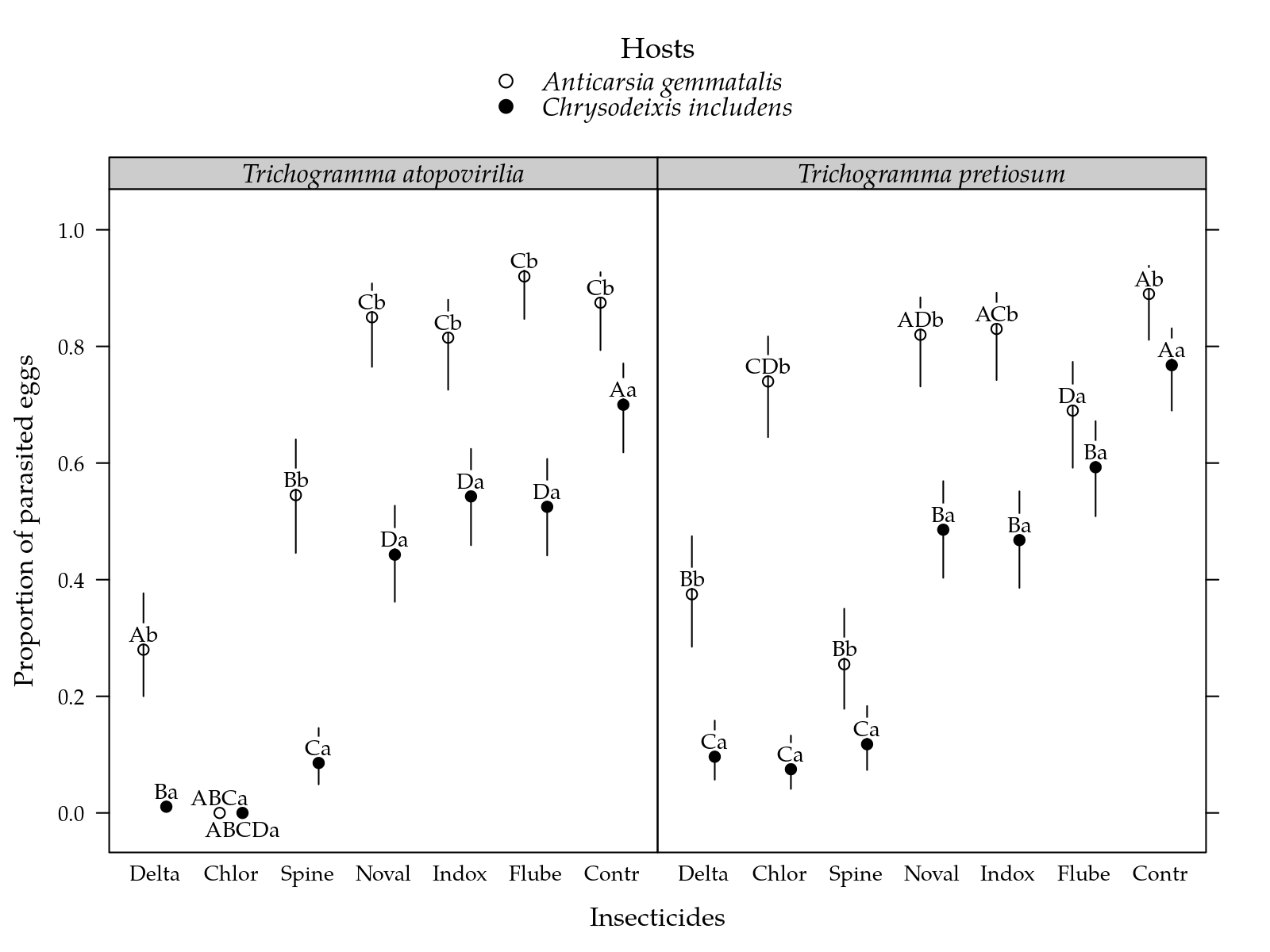
Figura 2: Estimated proportion of of parasitated eggs for each inseticide on two parasiods and two hosts. Segment is a confidence interval for the probability of surviving. Parasitoids estimates followed by the same lower letters in a insetice and host combination are not different at 5%. Inseticides estimates followed by the same lower letters in a parasitoid and host combination are not different at 5%.
Ovos Emergidos
#-----------------------------------------------------------------------
# Análise exploratória.

ftable(xtabs(!is.na(oeme) ~ I + P + H, data = egg))
## H Anti Chry
## I P
## Chlor Atopo 0 0
## Preti 19 6
## Delta Atopo 18 3
## Preti 19 15
## Spine Atopo 19 11
## Preti 17 17
## Flube Atopo 20 19
## Preti 19 19
## Indox Atopo 20 18
## Preti 19 20
## Noval Atopo 20 20
## Preti 20 20
## Contr Atopo 20 20
## Preti 20 20# ATTENTION: Com os 7 inseticidas dá cela perdida.
useOuterStrips(xyplot(oeme/opar ~ I | H + P,
data = egg[!is.na(egg$oeme), ],
jitter.x = TRUE,
type = c("p", "a")))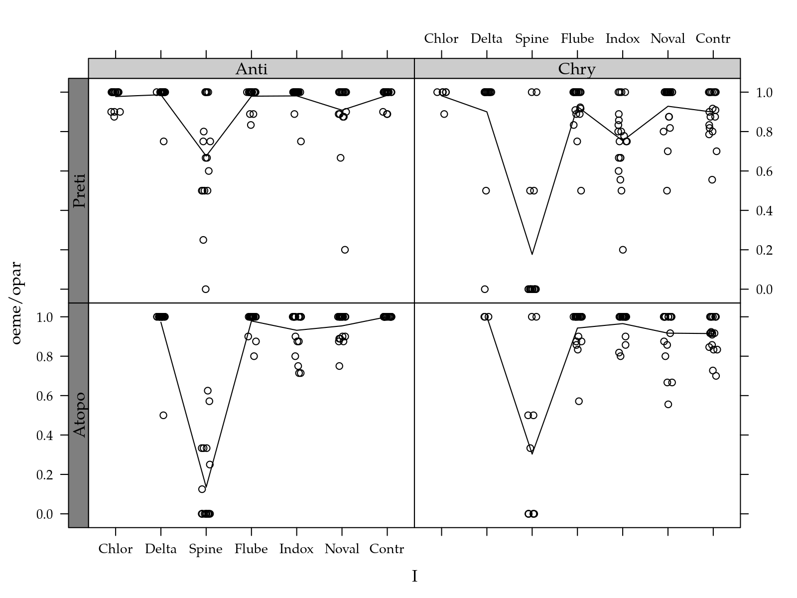
#-----------------------------------------------------------------------
# Ajuste do modelo.

m0 <- glm(cbind(oeme, opar - oeme) ~ I * P * H,
          data = egg,
          family = quasibinomial)

par(mfrow = c(2, 2))
plot(m0)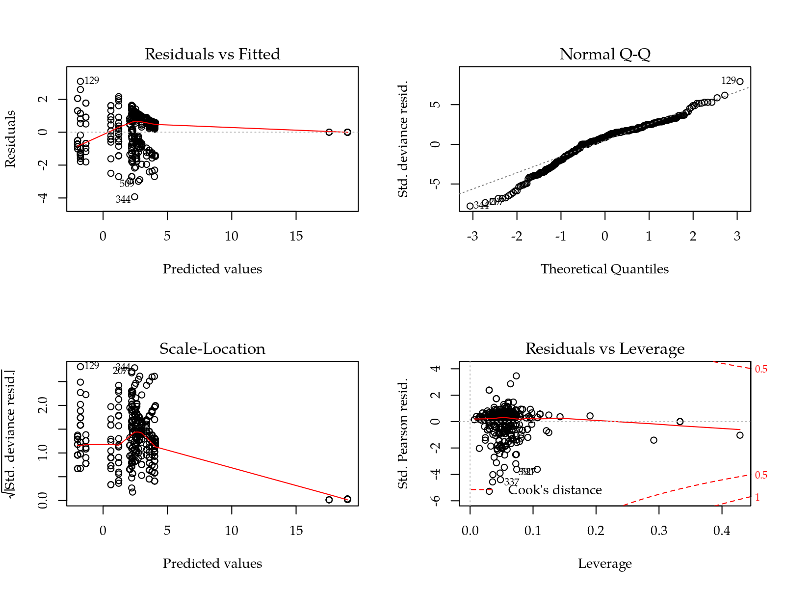
## Analysis of Deviance Table
##
## Model: quasibinomial, link: logit
##
## Response: cbind(oeme, opar - oeme)
##
## Terms added sequentially (first to last)
##
##
##       Df Deviance Resid. Df Resid. Dev       F    Pr(>F)
## NULL                    457    1189.96
## I      6   574.96       451     615.01 72.8264 < 2.2e-16 ***
## P      1     0.01       450     615.00  0.0053 0.9421318
## H      1    47.13       449     567.87 35.8188 4.553e-09 ***
## I:P    5    37.72       444     530.15  5.7334 3.891e-05 ***
## I:H    6    14.96       438     515.19  1.8947 0.0803009 .
## P:H    1     7.86       437     507.33  5.9730 0.0149254 *
## I:P:H  5    33.83       432     473.51  5.1415 0.0001358 ***
## ---
## Signif. codes:  0 '***' 0.001 '**' 0.01 '*' 0.05 '.' 0.1 ' ' 1
# Modelo declarado com a matrix do modelo, apenas os efeitos estimáveis.
X <- model.matrix(formula(m0)[-2], data = egg)
b <- coef(m0)
X <- X[, !is.na(b)]
m0 <- update(m0, . ~ 0 + X)
#-----------------------------------------------------------------------
# Comparações entre hospedeiros dentro de inseticida x parasitóide.
comp <- vector(mode = "list", length = 2)
# Declarar um modelo não deficiente aqui apenas para pegar a matriz.
lsm <- LE_matrix(lm(mort ~ I * P * H, data = egg),
effect = c("I", "P", "H"))
grid <- equallevels(attr(lsm, "grid"), egg)
# Celas que serão mantidas pois são estimaveis.
keep <- xtabs(!is.na(oeme) ~ interaction(I, P, H), data = egg) > 0
i <- with(grid, interaction(I, P, H) %in% names(keep[keep]))
grid <- grid[i, ]
lsm <- lsm[i, ]
# Deixa apenas as colunas de efeitos estimados.
lsm <- lsm[, !is.na(b)]
# Fazer as comparações apenas onde é possível.
# Hospedeiros dentro de inseticida x parasitóide.
rownames(lsm) <- grid$H
L <- by(lsm, INDICES = with(grid, interaction(I, P)), FUN = as.matrix)
i <- sapply(L, is.null)
L <- L[!i]
cmp <- lapply(L, apmc, model = m0, focus = "H", cld2 = TRUE)
pred <- ldply(cmp)
cmp <- ldply(strsplit(pred$.id, "\\."))
pred <- cbind(as.data.frame(cmp), pred[, -1])
names(pred)[1:2] <- c("I", "P")
names(pred)[ncol(pred)] <- "cldH"
comp[[1]] <- pred
# Fazer as comparações apenas onde é possível.
# Inseticidas dentro de parasitóide e hospedeiro.
rownames(lsm) <- grid$I
L <- by(lsm, INDICES = with(grid, interaction(H, P)), FUN = as.matrix)
cmp <- lapply(L, apmc, model = m0, focus = "I", test = "fdr",
cld2 = TRUE)
pred <- ldply(cmp)
cmp <- ldply(strsplit(pred$.id, "\\."))
pred <- cbind(as.data.frame(cmp), pred[, -1])
names(pred)[1:2] <- c("H", "P")
names(pred)[ncol(pred)] <- "cldI"
pred[, ncol(pred)] <- toupper(pred[, ncol(pred)])
comp[[2]] <- pred
str(comp)## List of 2
## $ :'data.frame': 26 obs. of 7 variables:
## ..$ I : chr [1:26] "Delta" "Delta" "Spine" "Spine" ...
## ..$ P : chr [1:26] "Atopo" "Atopo" "Atopo" "Atopo" ...
## ..$ H : Factor w/ 26 levels "Anti","Chry",..: 1 2 3 4 5 6 7 8 9 10 ...
## ..$ fit : num [1:26] 4.01 17.57 -1.76 -1.34 3.81 ...
## ..$ lwr : num [1:26] 1.74 -5117.68 -2.37 -2.47 2.67 ...
## ..$ upr : num [1:26] 6.276 5152.81 -1.152 -0.205 4.943 ...
## ..$ cldH: chr [1:26] "a" "a" "a" "a" ...
## $ :'data.frame': 26 obs. of 7 variables:
## ..$ H : chr [1:26] "Anti" "Anti" "Anti" "Anti" ...
## ..$ P : chr [1:26] "Atopo" "Atopo" "Atopo" "Atopo" ...
## ..$ I : Factor w/ 26 levels "Contr","Delta",..: 2 6 3 4 5 1 8 12 9 10 ...
## ..$ fit : num [1:26] 4.01 -1.76 3.81 2.63 3.01 ...
## ..$ lwr : num [1:26] 1.74 -2.37 2.67 1.92 2.19 ...
## ..$ upr : num [1:26] 6.28 -1.15 4.94 3.33 3.82 ...
## ..$ cldI: chr [1:26] "B" "A" "B" "B" ...pred <- merge(comp[[1]],
comp[[2]],
by = intersect(names(comp[[1]]), names(comp[[2]])))
pred$cld <- with(pred, paste(cldI, cldH, sep = ""))
#-----------------------------------------------------------------------
# Passa para a escala de probabilidade.
i <- c("fit", "lwr", "upr")
pred[, i] <- sapply(pred[, i], m0$family$linkinv)
# Ordena da tabela.
pred <- pred[with(pred, order(P, I, H)), ]
# Intervalos de confiança do tamanho do suporte terão apenas o ponto
# representado.
i <- pred$upr - pred$lwr > 0.99
if (any(i)) {
pred[i, ]$lwr <- pred[i, ]$lwr <- NA
}
# Reordena os níveis pela probalidade de sobreviência.
pred$I <- reorder(pred$I, pred$fit)
ftable(xtabs(~I + P + H, data = pred))## H Anti Chry Anti.1 Chry.1 Anti.2 Chry.2 Anti.3 Chry.3 Anti.4 Chry.4 Anti.5 Chry.5 Anti.6 Chry.6 Anti.7 Chry.7 Anti.8 Chry.8 Anti.9 Chry.9 Anti.10 Chry.10 Anti.11 Chry.11 Anti.12 Chry.12
## I P
## Delta Atopo 1 0 0 0 0 0 0 0 0 0 0 0 0 0 0 0 0 0 0 0 0 0 0 0 0 0# Legenda.
key <- list(points = list(pch = c(1, 19)),
text = list(levels(egg_parasitoid$hosp), font = 3),
title = "Hosts", cex.title = 1.1)
#-----------------------------------------------------------------------
ab <- aggregate(cbind(emerg = oeme/opar) ~ I + H + P,
data = egg,
FUN = mean)
kable(merge(pred, ab, by = intersect(names(pred), names(ab)))[, -c(5:9)])| I | P | H | fit | emerg |
|---|---|---|---|---|
| Delta | Atopo | Anti | 0.9821429 | 0.9722222 |
cap <-
"Estimated proportion of egg emergency for each inseticide on two parasiods and two hosts. Segment is a confidence interval for the probability of surviving. Parasitoids estimates followed by the same lower letters in a insetice and host combination are not different at 5%. Inseticides estimates followed by the same lower letters in a parasitoid and host combination are not different at 5%."
cap <- fgn_("oeme", cap)
# Gráfico de segmentos.
segplot(I ~ lwr + upr | P,
centers = fit,
data = pred,
xlab = "Insecticides",
ylab = "Probability of egg emergency",
draw = FALSE,
horizontal = FALSE,
groups = H,
key = key,
strip = strip.custom(
factor.levels = levels(egg_parasitoid$paras),
par.strip.text = list(font = 3)),
gap = 0.15,
cld = pred$cld,
panel = panel.groups.segplot,
pch = key$points$pch[as.integer(pred$H)]) +
layer({
a <- cld[which.max(nchar(cld))]
l <- cld[subscripts]
x <- as.integer(z)[subscripts] + centfac(groups[subscripts], gap)
y <- centers[subscripts]
# Usa símbolo unicode:
# http://www.alanwood.net/unicode/geometric_shapes.html
grid.text("\u25AE",
x = unit(x, "native"),
y = unit(y, "native"),
vjust = -0.5,
gp = gpar(col = "white")
)
grid.text(l,
x = unit(x, "native"),
y = unit(y, "native"),
vjust = -0.5,
gp = gpar(col = "black", fontsize = 10))
})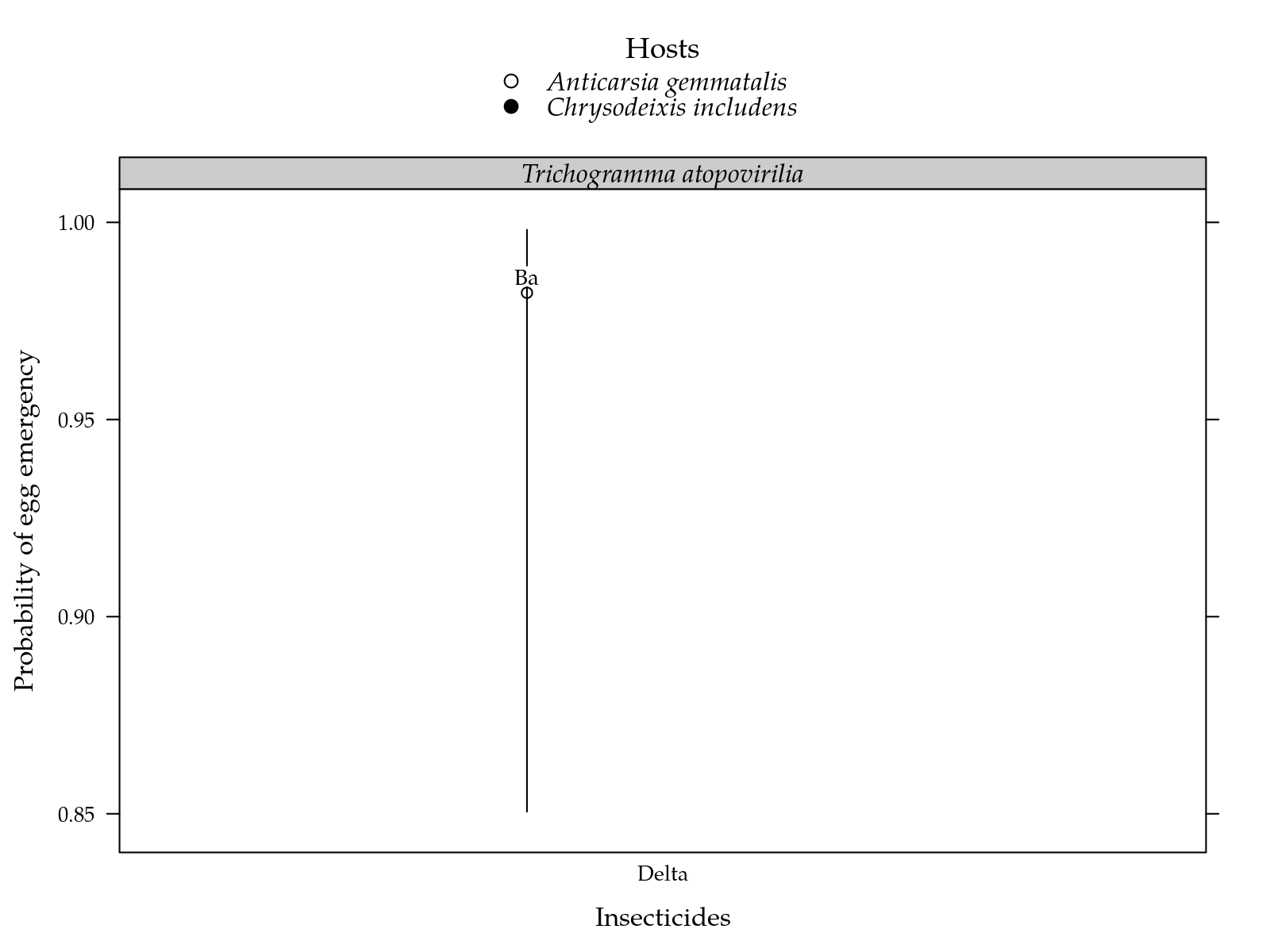
Figura 3: Estimated proportion of egg emergency for each inseticide on two parasiods and two hosts. Segment is a confidence interval for the probability of surviving. Parasitoids estimates followed by the same lower letters in a insetice and host combination are not different at 5%. Inseticides estimates followed by the same lower letters in a parasitoid and host combination are not different at 5%.
Tempo de Incubação dos Parasitóides
Essa variável apresenta pouca variação para algumas celas, portanto não informação suficiente para ser analisada.
Razão Sexual
#-----------------------------------------------------------------------
# Análise exploratória.
useOuterStrips(xyplot(femea + macho ~ I | H + P,
data = egg[!is.na(egg$macho + egg$femea), ],
jitter.x = TRUE,
auto.key = TRUE,
type = c("p", "a")))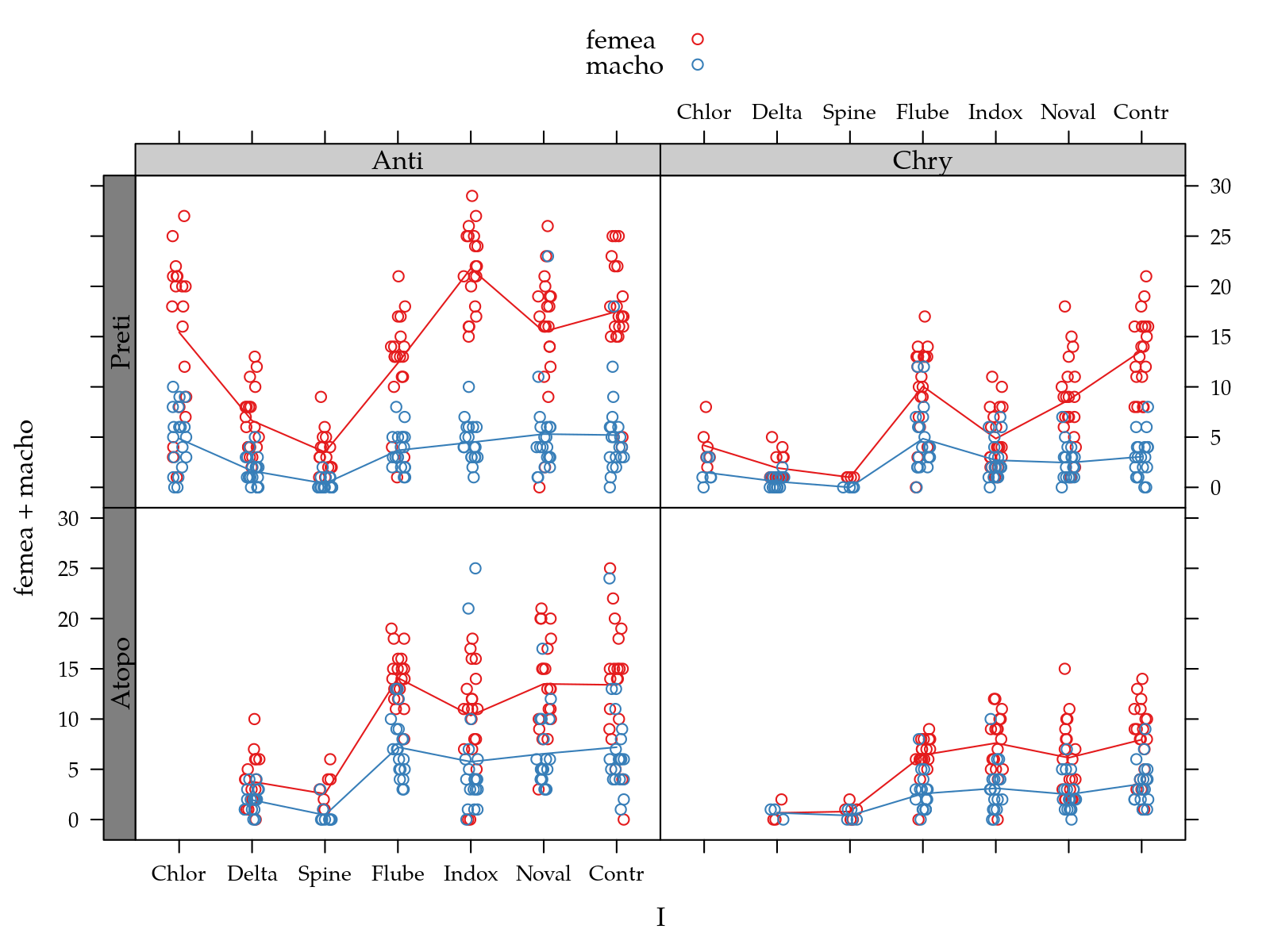
#-----------------------------------------------------------------------
# Ajuste do modelo.
m0 <- glm(cbind(femea, macho) ~ I * P * H,
data = egg,
family = quasibinomial)
par(mfrow = c(2, 2))
plot(m0)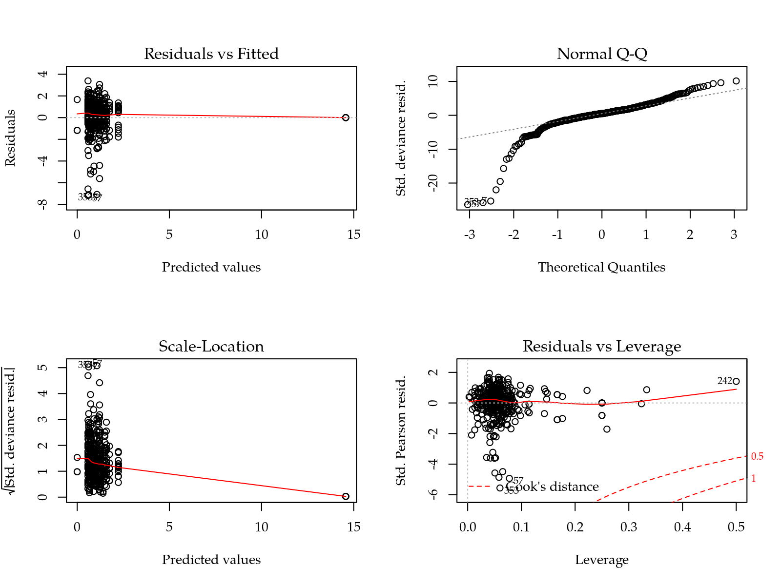
## Analysis of Deviance Table
##
## Model: quasibinomial, link: logit
##
## Response: cbind(femea, macho)
##
## Terms added sequentially (first to last)
##
##
## Df Deviance Resid. Df Resid. Dev F Pr(>F)
## NULL 426 979.85
## I 6 20.920 420 958.93 1.7374 0.11095
## P 1 60.370 419 898.56 30.0824 7.345e-08 ***
## H 1 0.037 418 898.52 0.0184 0.89218
## I:P 5 8.410 413 890.11 0.8382 0.52316
## I:H 6 11.008 407 879.10 0.9142 0.48445
## P:H 1 9.695 406 869.41 4.8309 0.02852 *
## I:P:H 5 20.116 401 849.29 2.0048 0.07702 .
## ---
## Signif. codes: 0 '***' 0.001 '**' 0.01 '*' 0.05 '.' 0.1 ' ' 1# summary(m0)
m1 <- glm(cbind(femea, macho) ~ P * H,
data = egg,
family = quasibinomial)
par(mfrow = c(2, 2))
plot(m1)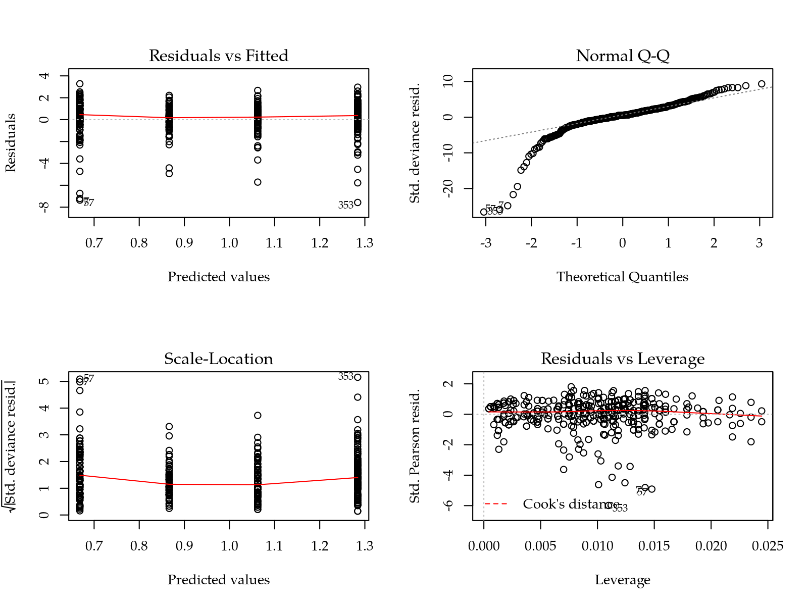
## Analysis of Deviance Table
##
## Model 1: cbind(femea, macho) ~ I * P * H
## Model 2: cbind(femea, macho) ~ P * H
## Resid. Df Resid. Dev Df Deviance F Pr(>F)
## 1 401 849.29
## 2 423 903.33 -22 -54.033 1.2238 0.2227anova(m1, test = "F")## Analysis of Deviance Table
##
## Model: quasibinomial, link: logit
##
## Response: cbind(femea, macho)
##
## Terms added sequentially (first to last)
##
##
## Df Deviance Resid. Df Resid. Dev F Pr(>F)
## NULL 426 979.85
## P 1 65.575 425 914.27 31.9573 2.903e-08 ***
## H 1 0.154 424 914.12 0.0753 0.7839
## P:H 1 10.795 423 903.33 5.2606 0.0223 *
## ---
## Signif. codes: 0 '***' 0.001 '**' 0.01 '*' 0.05 '.' 0.1 ' ' 1# summary(m1)
#-----------------------------------------------------------------------
# Comparações entre hospedeiros dentro de inseticida x parasitóide.
lsm <- LE_matrix(m1, effect = c("P", "H"))
grid <- equallevels(attr(lsm, "grid"), egg)
L <- by(lsm, INDICES = with(grid, P), FUN = as.matrix)
L <- lapply(L, "rownames<-", levels(egg$H))
cmp <- lapply(L, apmc, model = m1, focus = "H", cld2 = TRUE)
pred <- ldply(cmp)
# cmp <- ldply(strsplit(pred$.id, "\\."))
# pred <- cbind(as.data.frame(cmp), pred[, -1])
names(pred)[1] <- names(grid)[1]
pred <- equallevels(pred, egg)
# Passa para a escala de probabilidade.
i <- c("fit", "lwr", "upr")
pred[, i] <- sapply(pred[, i], m0$family$linkinv)
# Ordena da tabela.
pred <- pred[with(pred, order(P, H)), ]
# Intervalos de confiança do tamanho do suporte terão apenas o ponto
# representado.
i <- pred$upr - pred$lwr > 0.99
if (any(i)) {
pred[i, ]$lwr <- pred[i, ]$lwr <- NA
}
# Legenda.
key <- list(points = list(pch = c(1, 19)),
text = list(levels(egg_parasitoid$hosp), font = 3),
title = "Hosts", cex.title = 1.1)cap <-
"Estimated proportion of female parasitoids for each inseticide on two parasiods and two hosts. Segment is a confidence interval for the probability of surviving. Parasitoids estimates followed by the same lower letters in a insetice and host combination are not different at 5%. Inseticides estimates followed by the same lower letters in a parasitoid and host combination are not different at 5%."
cap <- fgn_("sexratio", cap)
# Gráfico de segmentos.
segplot(P ~ lwr + upr,
centers = fit,
data = pred,
xlab = "Parasitoids species",
ylab = "Proportion of female parasitoids",
draw = FALSE,
horizontal = FALSE,
groups = H,
key = key,
gap = 0.15,
cld = pred$cld,
panel = panel.groups.segplot,
pch = key$points$pch[as.integer(pred$H)]) +
layer({
a <- cld[which.max(nchar(cld))]
l <- cld[subscripts]
x <- as.integer(z)[subscripts] + centfac(groups[subscripts], gap)
y <- centers[subscripts]
# Usa símbolo unicode:
# http://www.alanwood.net/unicode/geometric_shapes.html
grid.text("\u25AE",
x = unit(x, "native"),
y = unit(y, "native"),
vjust = -0.5,
gp = gpar(col = "white")
)
grid.text(l,
x = unit(x, "native"),
y = unit(y, "native"),
vjust = -0.5,
gp = gpar(col = "black", fontsize = 10))
})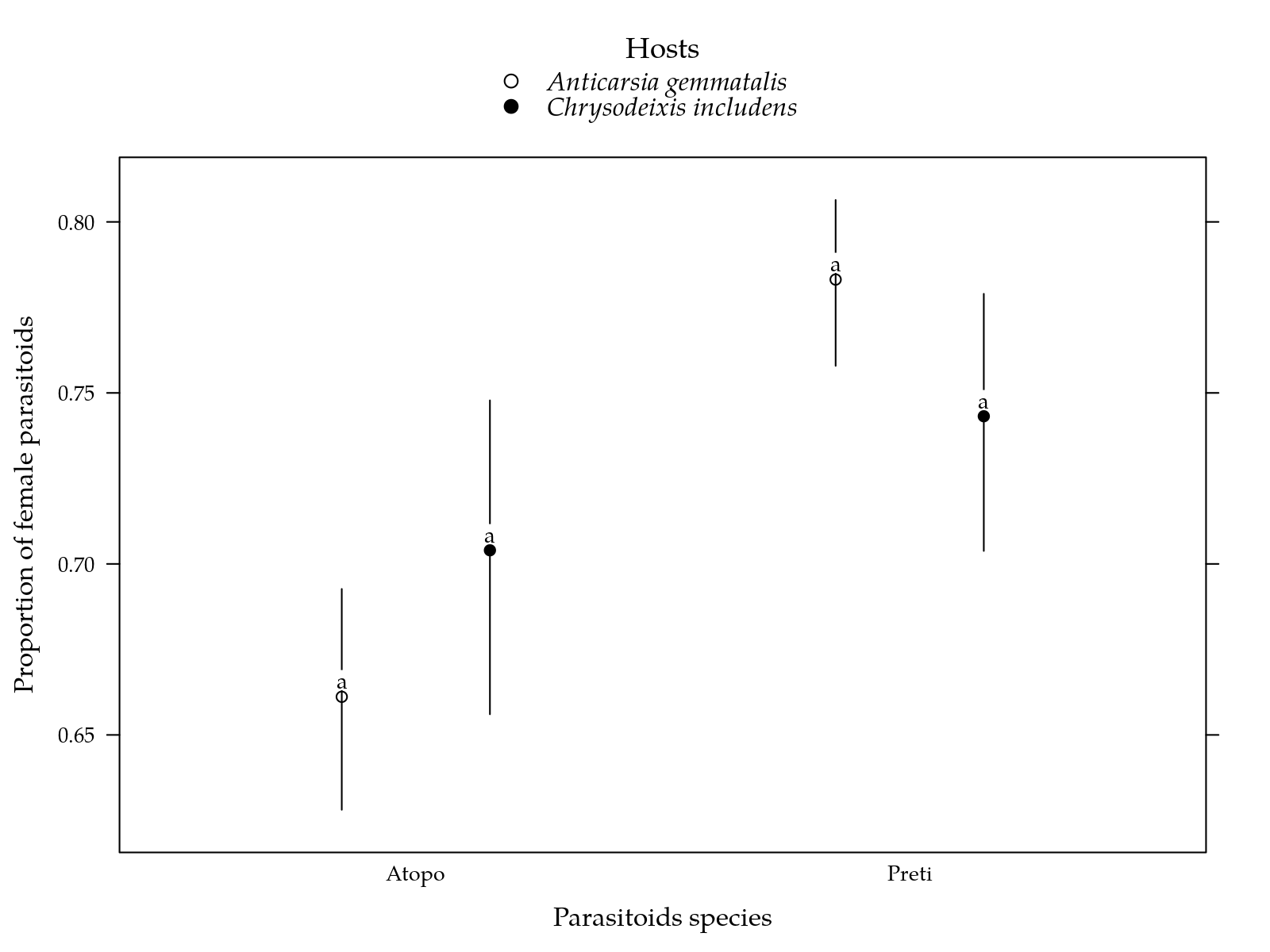
Figura 4: Estimated proportion of female parasitoids for each inseticide on two parasiods and two hosts. Segment is a confidence interval for the probability of surviving. Parasitoids estimates followed by the same lower letters in a insetice and host combination are not different at 5%. Inseticides estimates followed by the same lower letters in a parasitoid and host combination are not different at 5%.
Razão de Emergência dos Parasitóides
#-----------------------------------------------------------------------
# Análise exploratória.
egg$pem <- with(egg, femea + macho)
useOuterStrips(xyplot(pem + pne ~ I | H + P,
data = egg[!is.na(egg$pem + egg$pne), ],
jitter.x = TRUE,
auto.key = TRUE,
type = c("p", "a")))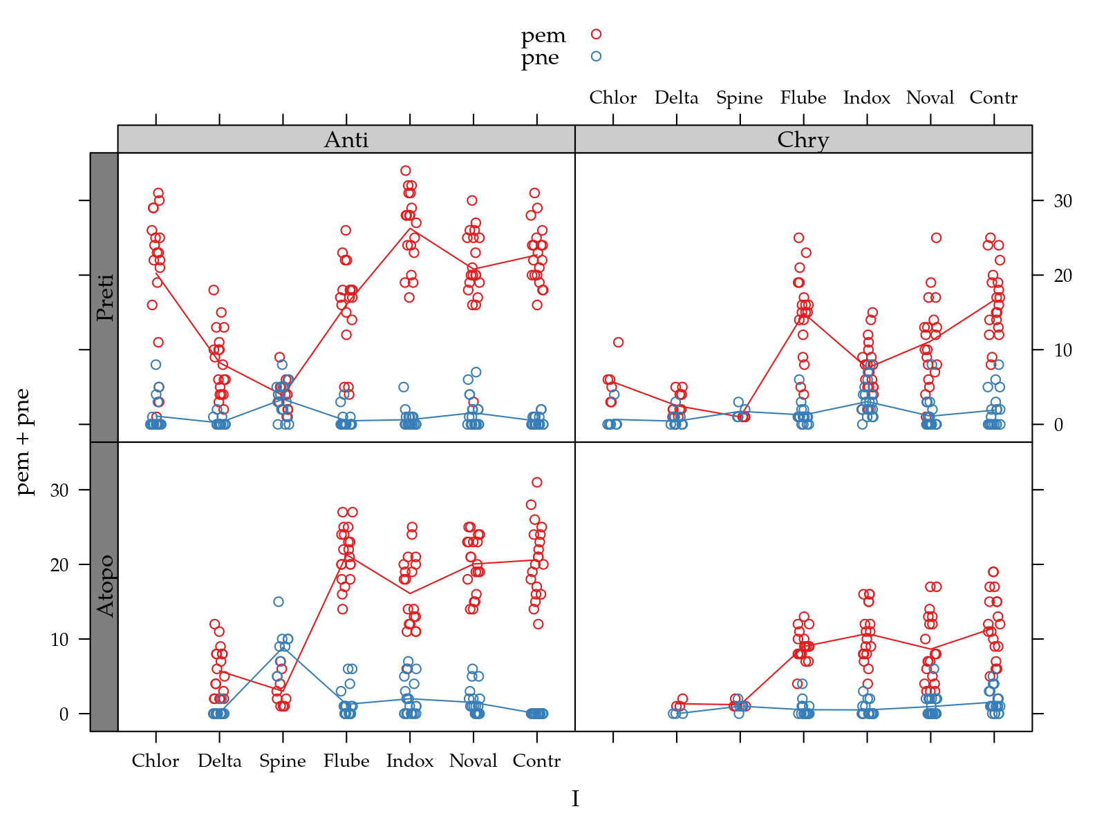
#-----------------------------------------------------------------------
# Ajuste do modelo.
m0 <- glm(cbind(pem, pne) ~ I * P * H,
data = egg,
family = quasibinomial)
par(mfrow = c(2, 2))
plot(m0)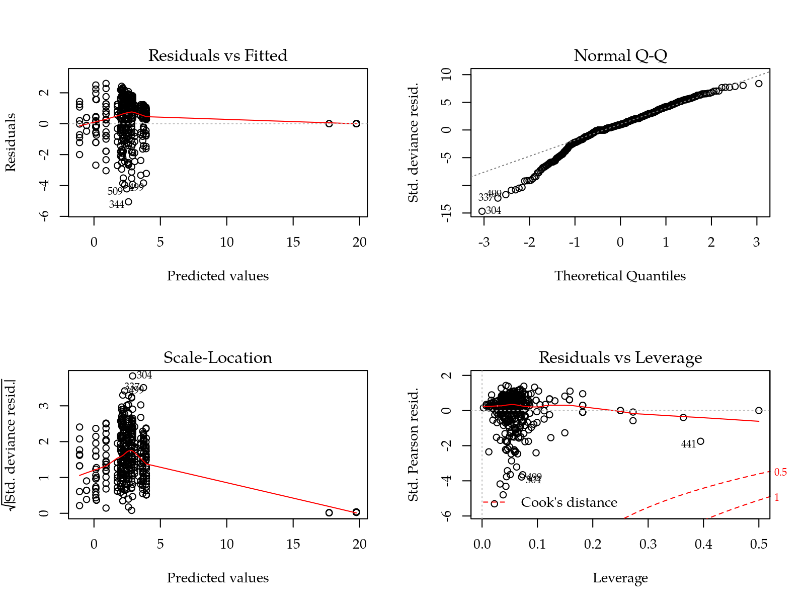
## Analysis of Deviance Table
##
## Model: quasibinomial, link: logit
##
## Response: cbind(pem, pne)
##
## Terms added sequentially (first to last)
##
##
## Df Deviance Resid. Df Resid. Dev F Pr(>F)
## NULL 426 1483.03
## I 6 466.81 420 1016.21 34.7674 < 2.2e-16 ***
## P 1 0.30 419 1015.91 0.1346 0.7138594
## H 1 83.60 418 932.31 37.3576 2.332e-09 ***
## I:P 5 18.31 413 914.00 1.6367 0.1491556
## I:H 6 46.38 407 867.63 3.4540 0.0024423 **
## P:H 1 29.06 406 838.57 12.9838 0.0003537 ***
## I:P:H 5 67.49 401 771.08 6.0321 2.130e-05 ***
## ---
## Signif. codes: 0 '***' 0.001 '**' 0.01 '*' 0.05 '.' 0.1 ' ' 1# summary(m0)
# Modelo declarado com a matrix do modelo, apenas os efeitos estimáveis.
X <- model.matrix(formula(m0)[-2], data = egg)
b <- coef(m0)
X <- X[, !is.na(b)]
m0 <- update(m0, . ~ 0 + X)

#-----------------------------------------------------------------------
# Comparações entre hospedeiros dentro de inseticida x parasitóide.

comp <- vector(mode = "list", length = 2)

# Declarar um modelo não deficiente aqui apenas para pegar a matriz.
lsm <- LE_matrix(lm(mort ~ I * P * H, data = egg),
                 effect = c("I", "P", "H"))
grid <- equallevels(attr(lsm, "grid"), egg)

# Celas que serão mantidas pois são estimaveis.
keep <- xtabs(!is.na(oeme) ~ interaction(I, P, H), data = egg) > 0
i <- with(grid, interaction(I, P, H) %in% names(keep[keep]))

grid <- grid[i, ]
lsm <- lsm[i, ]

# Deixa apenas as colunas de efeitos estimados.
lsm <- lsm[, !is.na(b)]

# Fazer as comparações apenas onde é possível.
# Hospedeiros dentro de inseticida x parasitóide.
rownames(lsm) <- grid$H
L <- by(lsm, INDICES = with(grid, interaction(I, P)), FUN = as.matrix)
i <- sapply(L, is.null)
L <- L[!i]

cmp <- lapply(L, apmc, model = m0, focus = "H", cld2 = TRUE)

pred <- ldply(cmp)
cmp <- ldply(strsplit(pred$.id, "\\."))
pred <- cbind(as.data.frame(cmp), pred[, -1])
names(pred)[1:2] <- c("I", "P")
names(pred)[ncol(pred)] <- "cldH"

comp[[1]] <- pred

# Fazer as comparações apenas onde é possível.
# Inseticidas dentro de parasitóide e hospedeiro.
rownames(lsm) <- grid$I
L <- by(lsm, INDICES = with(grid, interaction(H, P)), FUN = as.matrix)

cmp <- lapply(L, apmc, model = m0, focus = "I", test = "fdr",
              cld2 = TRUE)

pred <- ldply(cmp)
cmp <- ldply(strsplit(pred$.id, "\\."))
pred <- cbind(as.data.frame(cmp), pred[, -1])
names(pred)[1:2] <- c("H", "P")
names(pred)[ncol(pred)] <- "cldI"
pred[, ncol(pred)] <- toupper(pred[, ncol(pred)])

comp[[2]] <- pred
str(comp)
## List of 2
## $ :'data.frame': 26 obs. of 7 variables:
## ..$ I : chr [1:26] "Delta" "Delta" "Spine" "Spine" ...
## ..$ P : chr [1:26] "Atopo" "Atopo" "Atopo" "Atopo" ...
## ..$ H : Factor w/ 26 levels "Anti","Chry",..: 1 2 3 4 5 6 7 8 9 10 ...
## ..$ fit : num [1:26] 3.942 17.707 -1.086 0.182 2.836 ...
## ..$ lwr : num [1:26] 1.85 -6206.59 -1.74 -1.59 2.23 ...
## ..$ upr : num [1:26] 6.035 6242.005 -0.434 1.958 3.439 ...
## ..$ cldH: chr [1:26] "a" "a" "a" "a" ...
## $ :'data.frame': 26 obs. of 7 variables:
## ..$ H : chr [1:26] "Anti" "Anti" "Anti" "Anti" ...
## ..$ P : chr [1:26] "Atopo" "Atopo" "Atopo" "Atopo" ...
## ..$ I : Factor w/ 26 levels "Contr","Delta",..: 2 6 3 4 5 1 8 12 9 10 ...
## ..$ fit : num [1:26] 3.94 -1.09 2.84 2.09 2.59 ...
## ..$ lwr : num [1:26] 1.85 -1.74 2.23 1.59 2.04 ...
## ..$ upr : num [1:26] 6.035 -0.434 3.439 2.577 3.148 ...
## ..$ cldI: chr [1:26] "B" "A" "B" "B" ...pred <- merge(comp[[1]],
comp[[2]],
by = intersect(names(comp[[1]]), names(comp[[2]])))
pred$cld <- with(pred, paste(cldI, cldH, sep = ""))
#-----------------------------------------------------------------------
# Passa para a escala de probabilidade.
i <- c("fit", "lwr", "upr")
pred[, i] <- sapply(pred[, i], m0$family$linkinv)
# Ordena da tabela.
pred <- pred[with(pred, order(P, I, H)), ]
# Intervalos de confiança do tamanho do suporte terão apenas o ponto
# representado.
i <- pred$upr - pred$lwr > 0.99
if (any(i)) {
pred[i, ]$lwr <- pred[i, ]$lwr <- NA
}
# Reordena os níveis pela probalidade de sobreviência.
pred$I <- reorder(pred$I, pred$fit)
# Legenda.
key <- list(points = list(pch = c(1, 19)),
text = list(levels(egg_parasitoid$hosp), font = 3),
title = "Hosts", cex.title = 1.1)cap <-
"Estimated parasitoid emergency proportion for each inseticide on two parasiods and two hosts. Segment is a confidence interval for the probability of surviving. Parasitoids estimates followed by the same lower letters in a insetice and host combination are not different at 5%. Inseticides estimates followed by the same lower letters in a parasitoid and host combination are not different at 5%."
cap <- fgn_("pemer", cap)
# Gráfico de segmentos.
segplot(I ~ lwr + upr | P,
centers = fit,
data = pred,
xlab = "Insecticides",
ylab = "Proportion of parasitoid emergency",
draw = FALSE,
horizontal = FALSE,
groups = H,
key = key,
strip = strip.custom(
factor.levels = levels(egg_parasitoid$paras),
par.strip.text = list(font = 3)),
gap = 0.15,
cld = pred$cld,
panel = panel.groups.segplot,
pch = key$points$pch[as.integer(pred$H)]) +
layer({
a <- cld[which.max(nchar(cld))]
l <- cld[subscripts]
x <- as.integer(z)[subscripts] + centfac(groups[subscripts], gap)
y <- centers[subscripts]
# Usa símbolo unicode:
# http://www.alanwood.net/unicode/geometric_shapes.html
grid.text("\u25AE",
x = unit(x, "native"),
y = unit(y, "native"),
vjust = -0.5,
gp = gpar(col = "white")
)
grid.text(l,
x = unit(x, "native"),
y = unit(y, "native"),
vjust = -0.5,
gp = gpar(col = "black", fontsize = 10))
})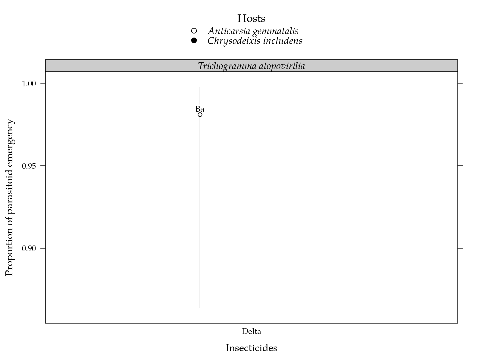
Figura 5: Estimated parasitoid emergency proportion for each inseticide on two parasiods and two hosts. Segment is a confidence interval for the probability of surviving. Parasitoids estimates followed by the same lower letters in a insetice and host combination are not different at 5%. Inseticides estimates followed by the same lower letters in a parasitoid and host combination are not different at 5%.
Total de Parasitóides
#-----------------------------------------------------------------------
# Análise exploratória.

egg$ptot <- with(egg, femea + macho + pne)

useOuterStrips(xyplot(ptot ~ I | H + P,
                      data = egg[!is.na(egg$ptot), ],
                      jitter.x = TRUE,
                      auto.key = TRUE,
                      type = c("p", "a")))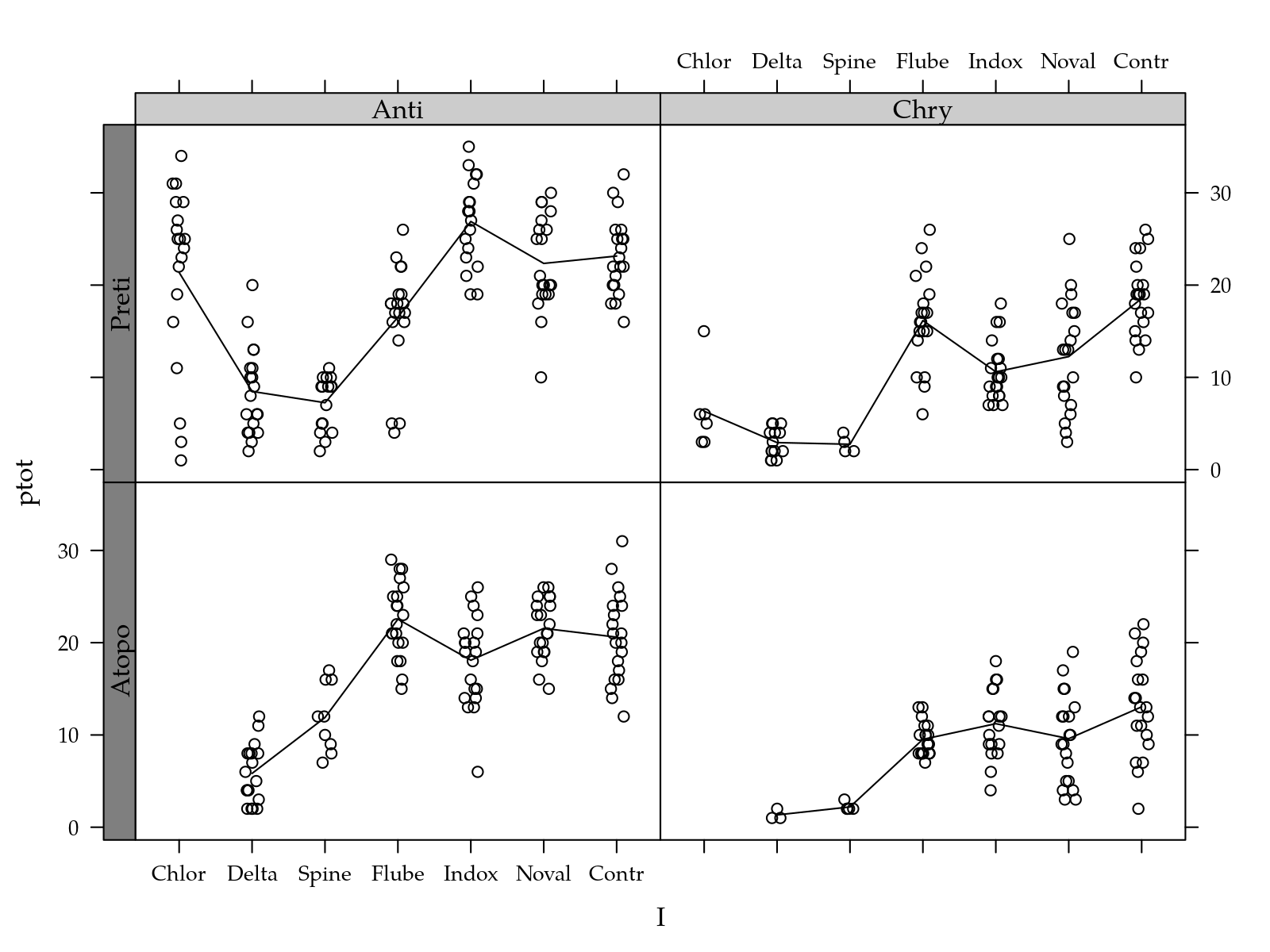
#-----------------------------------------------------------------------
# Ajuste do modelo.

m0 <- glm(ptot ~ I * P * H,
          data = egg,
          family = quasipoisson)

par(mfrow = c(2, 2))
plot(m0)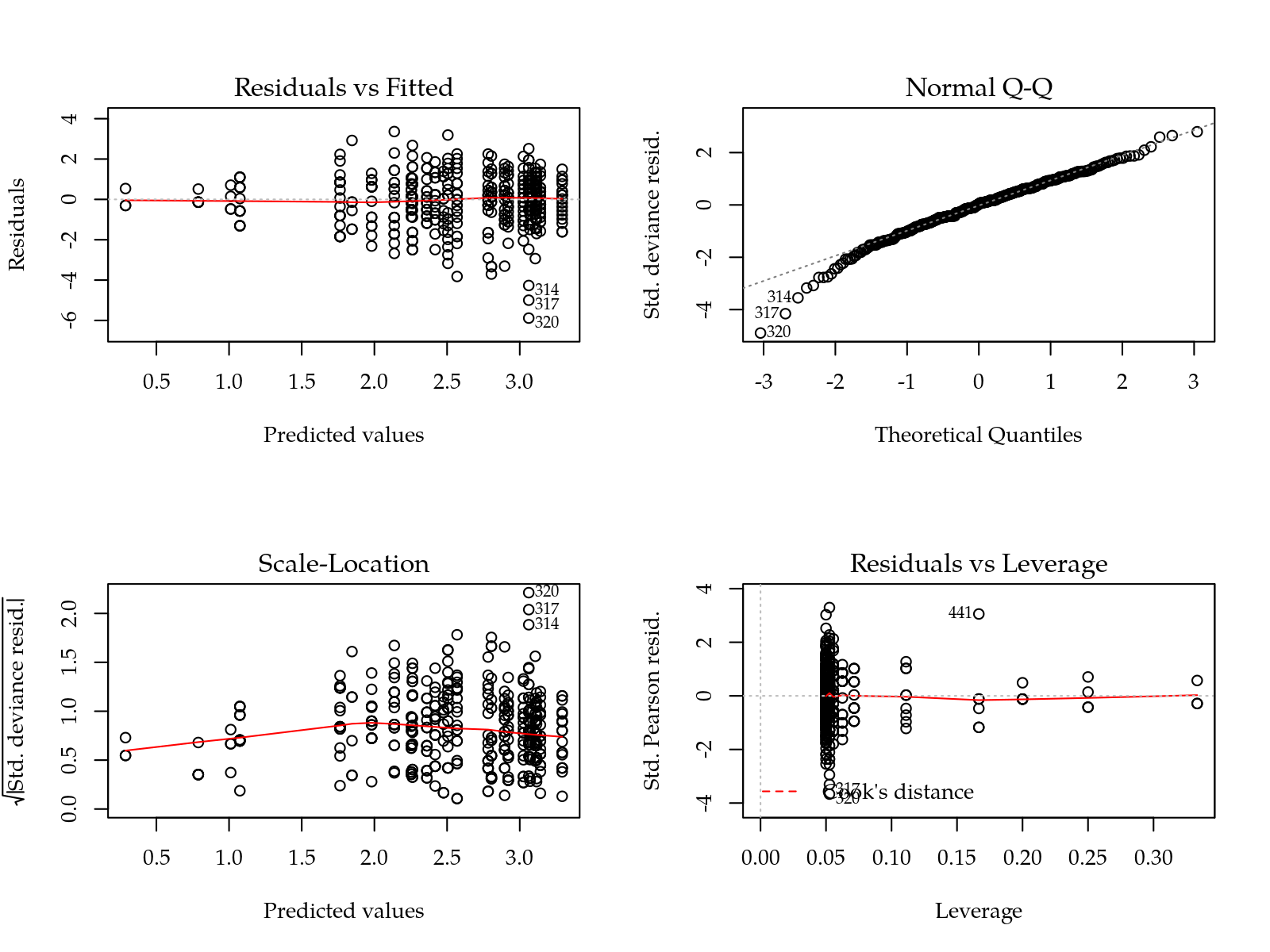
## Analysis of Deviance Table
##
## Model: quasipoisson, link: log
##
## Response: ptot
##
## Terms added sequentially (first to last)
##
##
##       Df Deviance Resid. Df Resid. Dev        F    Pr(>F)
## NULL                    426    2062.89
## I      6   690.95       420    1371.94  75.5155 < 2.2e-16 ***
## P      1    22.91       419    1349.03  15.0222 0.0001241 ***
## H      1   495.05       418     853.98 324.6323 < 2.2e-16 ***
## I:P    5    28.02       413     825.96   3.6755 0.0029022 **
## I:H    6    85.14       407     740.82   9.3056 1.458e-09 ***
## P:H    1    16.19       406     724.62  10.6184 0.0012151 **
## I:P:H  5    60.32       401     664.30   7.9116 4.014e-07 ***
## ---
## Signif. codes:  0 '***' 0.001 '**' 0.01 '*' 0.05 '.' 0.1 ' ' 1
# summary(m0)
# Modelo declarado com a matrix do modelo, apenas os efeitos estimáveis.
X <- model.matrix(formula(m0)[-2], data = egg)
b <- coef(m0)
X <- X[, !is.na(b)]
m0 <- update(m0, . ~ 0 + X)
#-----------------------------------------------------------------------
# Comparações entre hospedeiros dentro de inseticida x parasitóide.
comp <- vector(mode = "list", length = 2)
# Declarar um modelo não deficiente aqui apenas para pegar a matriz.
lsm <- LE_matrix(lm(mort ~ I * P * H, data = egg),
effect = c("I", "P", "H"))
grid <- equallevels(attr(lsm, "grid"), egg)
# Celas que serão mantidas pois são estimaveis.
keep <- xtabs(!is.na(oeme) ~ interaction(I, P, H), data = egg) > 0
i <- with(grid, interaction(I, P, H) %in% names(keep[keep]))
grid <- grid[i, ]
lsm <- lsm[i, ]
# Deixa apenas as colunas de efeitos estimados.
lsm <- lsm[, !is.na(b)]
# Fazer as comparações apenas onde é possível.
# Hospedeiros dentro de inseticida x parasitóide.
rownames(lsm) <- grid$H
L <- by(lsm, INDICES = with(grid, interaction(I, P)), FUN = as.matrix)
i <- sapply(L, is.null)
L <- L[!i]
cmp <- lapply(L, apmc, model = m0, focus = "H", cld2 = TRUE)
pred <- ldply(cmp)
cmp <- ldply(strsplit(pred$.id, "\\."))
pred <- cbind(as.data.frame(cmp), pred[, -1])
names(pred)[1:2] <- c("I", "P")
names(pred)[ncol(pred)] <- "cldH"
comp[[1]] <- pred
# Fazer as comparações apenas onde é possível.
# Inseticidas dentro de parasitóide e hospedeiro.
rownames(lsm) <- grid$I
L <- by(lsm, INDICES = with(grid, interaction(H, P)), FUN = as.matrix)
cmp <- lapply(L, apmc, model = m0, focus = "I", test = "fdr",
cld2 = TRUE)
pred <- ldply(cmp)
cmp <- ldply(strsplit(pred$.id, "\\."))
pred <- cbind(as.data.frame(cmp), pred[, -1])
names(pred)[1:2] <- c("H", "P")
names(pred)[ncol(pred)] <- "cldI"
pred[, ncol(pred)] <- toupper(pred[, ncol(pred)])
comp[[2]] <- pred
str(comp)## List of 2
## $ :'data.frame': 26 obs. of 7 variables:
## ..$ I : chr [1:26] "Delta" "Delta" "Spine" "Spine" ...
## ..$ P : chr [1:26] "Atopo" "Atopo" "Atopo" "Atopo" ...
## ..$ H : Factor w/ 26 levels "Anti","Chry",..: 1 2 3 4 5 6 7 8 9 10 ...
## ..$ fit : num [1:26] 1.764 0.288 2.476 0.788 3.116 ...
## ..$ lwr : num [1:26] 1.5274 -0.9225 2.2416 0.0587 3.0018 ...
## ..$ upr : num [1:26] 2 1.5 2.71 1.52 3.23 ...
## ..$ cldH: chr [1:26] "b" "a" "b" "a" ...
## $ :'data.frame': 26 obs. of 7 variables:
## ..$ H : chr [1:26] "Anti" "Anti" "Anti" "Anti" ...
## ..$ P : chr [1:26] "Atopo" "Atopo" "Atopo" "Atopo" ...
## ..$ I : Factor w/ 26 levels "Contr","Delta",..: 2 6 3 4 5 1 8 12 9 10 ...
## ..$ fit : num [1:26] 1.76 2.48 3.12 2.9 3.07 ...
## ..$ lwr : num [1:26] 1.53 2.24 3 2.77 2.95 ...
## ..$ upr : num [1:26] 2 2.71 3.23 3.02 3.19 ...
## ..$ cldI: chr [1:26] "D" "C" "B" "A" ...pred <- merge(comp[[1]],
comp[[2]],
by = intersect(names(comp[[1]]), names(comp[[2]])))
pred$cld <- with(pred, paste(cldI, cldH, sep = ""))
#-----------------------------------------------------------------------
# Passa para a escala de probabilidade.
i <- c("fit", "lwr", "upr")
pred[, i] <- sapply(pred[, i], m0$family$linkinv)
# Ordena da tabela.
pred <- pred[with(pred, order(P, I, H)), ]
# Reordena os níveis pela probalidade de sobreviência.
pred$I <- reorder(pred$I, pred$fit)
# Legenda.
key <- list(points = list(pch = c(1, 19)),
text = list(levels(egg_parasitoid$hosp), font = 3),
title = "Hosts", cex.title = 1.1)cap <-
"Estimated total number of parasitoids for each inseticide on two parasiods and two hosts. Segment is a confidence interval for the probability of surviving. Parasitoids estimates followed by the same lower letters in a insetice and host combination are not different at 5%. Inseticides estimates followed by the same lower letters in a parasitoid and host combination are not different at 5%."
cap <- fgn_("tot", cap)
# Gráfico de segmentos.
segplot(I ~ lwr + upr | P,
centers = fit,
data = pred,
xlab = "Insecticides",
ylab = "Total of parasitoids",
draw = FALSE,
horizontal = FALSE,
groups = H,
key = key,
strip = strip.custom(
factor.levels = levels(egg_parasitoid$paras),
par.strip.text = list(font = 3)),
gap = 0.15,
cld = pred$cld,
panel = panel.groups.segplot,
pch = key$points$pch[as.integer(pred$H)]) +
layer({
a <- cld[which.max(nchar(cld))]
l <- cld[subscripts]
x <- as.integer(z)[subscripts] + centfac(groups[subscripts], gap)
y <- centers[subscripts]
# Usa símbolo unicode:
# http://www.alanwood.net/unicode/geometric_shapes.html
grid.text("\u25AE",
x = unit(x, "native"),
y = unit(y, "native"),
vjust = -0.5,
gp = gpar(col = "white")
)
grid.text(l,
x = unit(x, "native"),
y = unit(y, "native"),
vjust = -0.5,
gp = gpar(col = "black", fontsize = 10))
})
Figura 6: Estimated total number of parasitoids for each inseticide on two parasiods and two hosts. Segment is a confidence interval for the probability of surviving. Parasitoids estimates followed by the same lower letters in a insetice and host combination are not different at 5%. Inseticides estimates followed by the same lower letters in a parasitoid and host combination are not different at 5%.
Session information
## quinta, 11 de julho de 2019, 20:05
## ----------------------------------------
## R version 3.6.1 (2019-07-05)
## Platform: x86_64-pc-linux-gnu (64-bit)
## Running under: Ubuntu 18.04.2 LTS
##
## Matrix products: default
## BLAS:   /usr/lib/x86_64-linux-gnu/blas/libblas.so.3.7.1
## LAPACK: /usr/lib/x86_64-linux-gnu/lapack/liblapack.so.3.7.1
##
## locale:
##  [1] LC_CTYPE=pt_BR.UTF-8       LC_NUMERIC=C
##  [3] LC_TIME=pt_BR.UTF-8        LC_COLLATE=en_US.UTF-8
##  [5] LC_MONETARY=pt_BR.UTF-8    LC_MESSAGES=en_US.UTF-8
##  [7] LC_PAPER=pt_BR.UTF-8       LC_NAME=C
##  [9] LC_ADDRESS=C               LC_TELEPHONE=C
## [11] LC_MEASUREMENT=pt_BR.UTF-8 LC_IDENTIFICATION=C
##
## attached base packages:
## [1] stats     graphics  grDevices utils     datasets  methods
## [7] base
##
## other attached packages:
##  [1] captioner_2.2.3     knitr_1.23          RDASC_0.0-6
##  [4] multcomp_1.4-10     TH.data_1.0-10      MASS_7.3-51.4
##  [7] survival_2.44-1.1   mvtnorm_1.0-11      doBy_4.6-2
## [10] plyr_1.8.4          latticeExtra_0.6-28 RColorBrewer_1.1-2
## [13] lattice_0.20-38     wzRfun_0.81
##
## loaded via a namespace (and not attached):
##  [1] Rcpp_1.0.1       highr_0.8        compiler_3.6.1
##  [4] pillar_1.4.2     tools_3.6.1      digest_0.6.20
##  [7] evaluate_0.14    memoise_1.1.0    tibble_2.1.3
## [10] pkgconfig_2.0.2  rlang_0.4.0      Matrix_1.2-17
## [13] commonmark_1.7   rpanel_1.1-4     yaml_2.2.0
## [16] pkgdown_1.3.0    xfun_0.8         stringr_1.4.0
## [19] dplyr_0.8.3      roxygen2_6.1.1   xml2_1.2.0
## [22] desc_1.2.0       fs_1.3.1         rprojroot_1.3-2
## [25] grid_3.6.1       tidyselect_0.2.5 glue_1.3.1
## [28] R6_2.4.0         tcltk_3.6.1      rmarkdown_1.13
## [31] purrr_0.3.2      magrittr_1.5     codetools_0.2-16
## [34] splines_3.6.1    backports_1.1.4  htmltools_0.3.6
## [37] assertthat_0.2.1 sandwich_2.5-1   stringi_1.4.3
## [40] crayon_1.3.4     zoo_1.8-6