Effect of fungicide sprays programs and pistachio hedging on incidende and severity caused by Alternaria late blight in commercial pistachio orchard of Tulare County, California
Paulo S. F. Lichtemberg, Ryan D. Puckett, Walmes M. Zeviani, Connor G. Cunningham & Themis J. Michailides
2019-07-11
ake_b-severity.RmdSession Definition
# https://github.com/walmes/wzRfun
# devtools::install_github("walmes/wzRfun")

library(lattice)
library(latticeExtra)
library(plyr)
library(reshape)
library(doBy)
library(multcomp)
library(lme4)
library(lmerTest)
library(wzRfun)library(RDASC)Exploratory data analysis
# Data strucuture.
str(ake_b$severity)
## 'data.frame': 192 obs. of 8 variables:
## $ yr : int 2015 2015 2015 2015 2015 2015 2015 2015 2015 2015 ...
## $ hed: Factor w/ 2 levels "heavy","normal": 1 1 1 1 2 2 2 2 1 1 ...
## $ tra: Factor w/ 4 levels "cnt","fon2","mer2",..: 4 4 4 1 2 2 2 1 3 3 ...
## $ plo: Factor w/ 12 levels "1A","1B","1C",..: 1 1 1 1 2 2 2 2 3 3 ...
## $ tre: int 1 2 3 4 5 6 7 8 9 10 ...
## $ rep: int 1 1 1 1 1 1 1 1 1 1 ...
## $ inc: num 4.8 4.8 4.5 4 3 3.5 4.5 2.8 5 4.5 ...
## $ def: int 2 20 8 6 10 16 3 35 9 10 ...# Short names are easier to use.
da <- ake_b$severity
da$yr <- factor(da$yr)
# Creating the blocks.
da$block <- with(da, {
factor(ifelse(as.integer(gsub("\\D", "", plo)) > 2, "II", "I"))
})
xtabs(~block, data = da)## block
## I II
## 96 96## hed heavy normal
## yr tra
## 2015 cnt 12 12
## fon2 12 12
## mer2 12 12
## mer3 12 12
## 2016 cnt 12 12
## fon2 12 12
## mer2 12 12
## mer3 12 12xtabs(~yr + rep, data = da)## rep
## yr 1 2
## 2015 48 48
## 2016 48 48combineLimits(
useOuterStrips(
xyplot(inc + def ~ tra | yr,
data = da,
outer = TRUE,
groups = hed,
type = c("p", "a"),
auto.key = TRUE,
jitter.x = TRUE,
xlab = "Fungicides",
ylab = "Incidence and defoliation",
scales = "free")))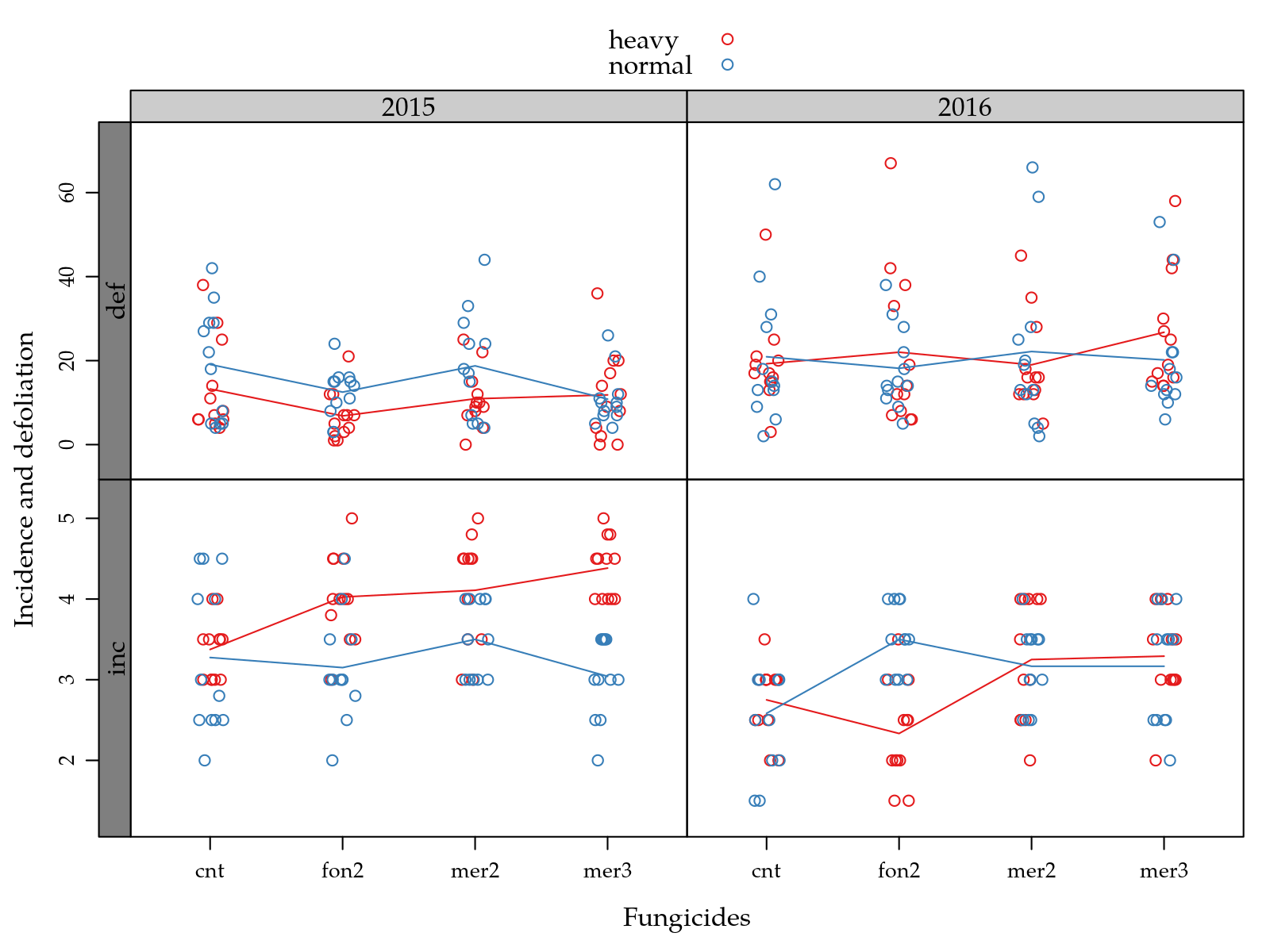
Severity
# Just to barely check the model assumptions.
m0 <- lm(inc ~ block + yr * tra * hed, data = da)
par(mfrow = c(2, 2))
plot(m0)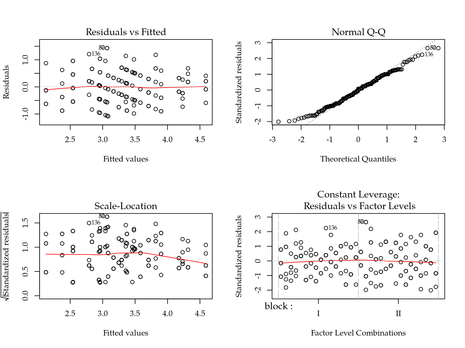
layout(1)

# No transformed.
da$y <- da$inc

# Mixed models.
m0 <- lmer(y ~ yr/block + (yr + tra + hed)^2 + (1 | tre),
           data = da)

anova(m0)
## Type III Analysis of Variance Table with Satterthwaite's method
## Sum Sq Mean Sq NumDF DenDF F value Pr(>F)
## yr 5.9296 5.9296 1 159.454 24.7477 1.676e-06 ***
## tra 2.7755 0.9252 3 71.005 3.8612 0.0128308 *
## hed 0.4624 0.4624 1 125.325 1.9300 0.1672181
## yr:block 4.1258 2.0629 2 144.349 8.6097 0.0002935 ***
## yr:tra 0.3347 0.1116 3 144.740 0.4657 0.7066984
## yr:hed 9.0873 9.0873 1 174.347 37.9268 4.922e-09 ***
## tra:hed 1.3835 0.4612 3 112.575 1.9247 0.1296208
## ---
## Signif. codes: 0 '***' 0.001 '**' 0.01 '*' 0.05 '.' 0.1 ' ' 1# summary(m0)# Fake model just to use the LE_matrix().
fake <- lm(nobars(formula(m0)), m0@frame)
cmp <- list()
# Main effect of fungicide.
L <- LE_matrix(fake, effect = "tra")
grid <- equallevels(attr(L, "grid"), da)
rownames(L) <- grid[, 1]
a <- apmc(X = L, model = m0, focus = "tra")
cmp$tra <- a
# Spliting the effect of head in each year.
L <- LE_matrix(fake, effect = c("yr", "hed"))
grid <- equallevels(attr(L, "grid"), da)
L <- by(L, grid$yr, as.matrix)
L <- lapply(L, "rownames<-", levels(grid$hed))
a <- ldply(lapply(L, apmc, model = m0, focus = "hed"), .id = "yr")
cmp$"yr:hed" <- ap1 <- segplot(tra ~ lwr + upr,
centers = fit,
data = cmp$tra,
draw = FALSE,
xlab = "Disease incidence",
ylab = "Fungicides",
ann = sprintf("%0.2f %s",
cmp$tra$fit,
cmp$tra$cld)) +
layer(panel.text(x = centers[subscripts],
y = z[subscripts],
labels = ann[subscripts],
pos = 3))
p2 <- segplot(hed ~ lwr + upr | yr,
centers = fit,
data = cmp$"yr:hed",
draw = FALSE,
layout = c(1, NA),
xlab = "Disease incidence",
ylab = "Hedging level",
as.table = TRUE,
ann = sprintf("%0.2f %s",
cmp$"yr:hed"$fit,
cmp$"yr:hed"$cld)) +
layer(panel.text(x = centers[subscripts],
y = z[subscripts],
labels = ann[subscripts],
pos = 3))
print(p1, position = c(0, 0.55, 1, 1), more = TRUE)
print(p2, position = c(0, 0, 1, 0.55))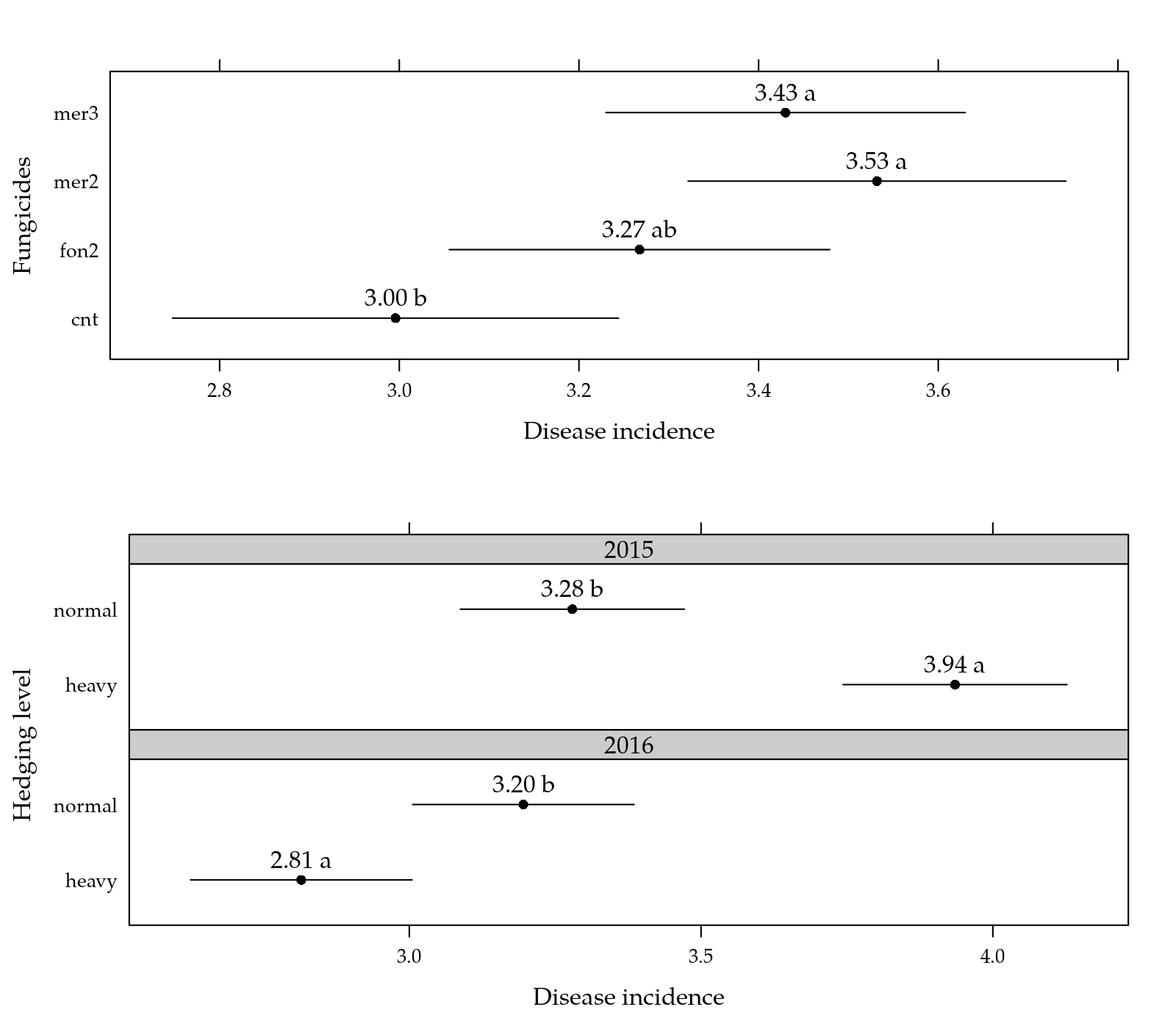
Figure 1: Mean incidence as function of each factor levels.
Defoliation
# Just to barely check the model assumptions.
m0 <- lm(def + 1 ~ block + yr * tra * hed, data = da)
par(mfrow = c(2, 2))
plot(m0)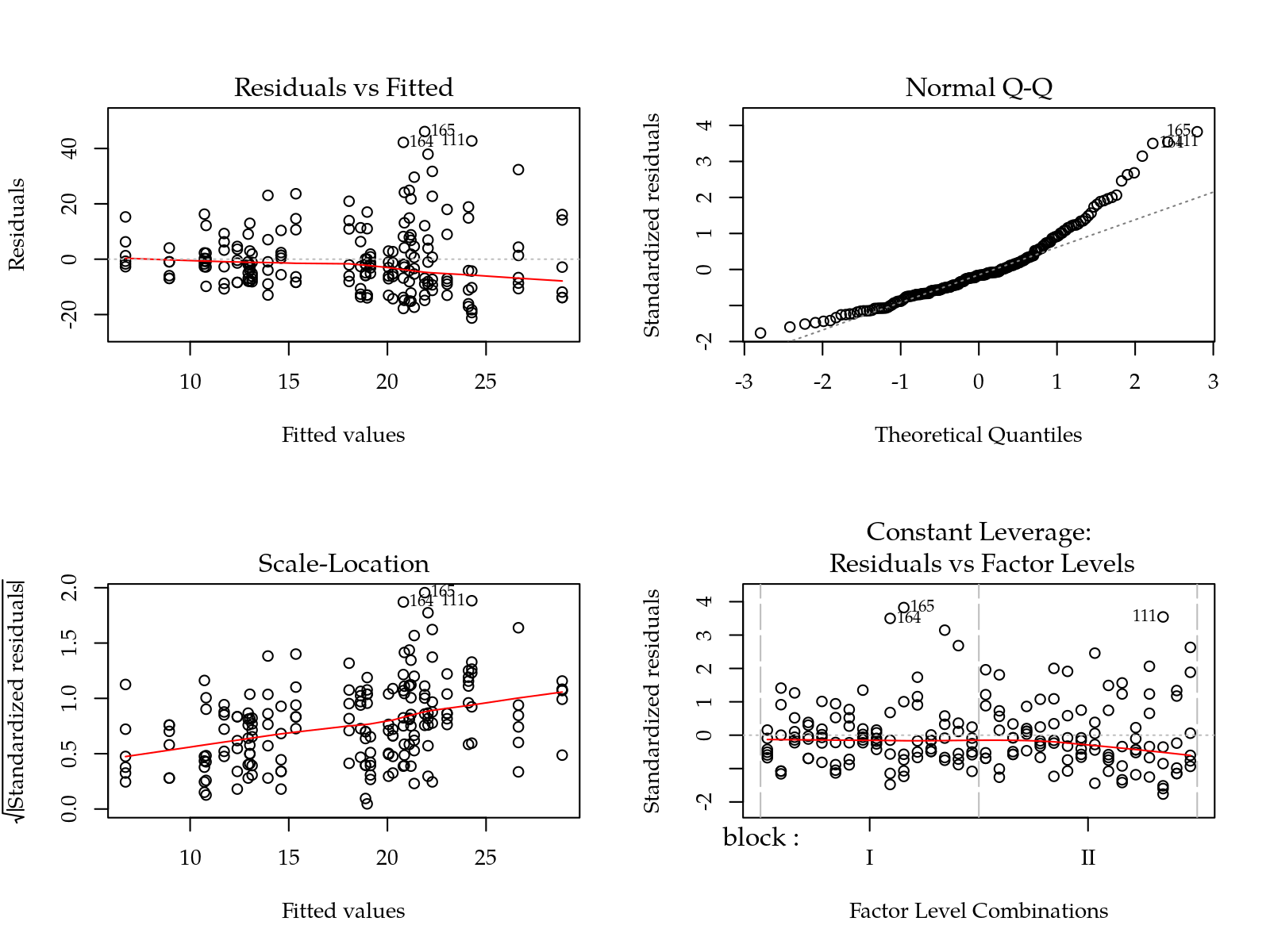
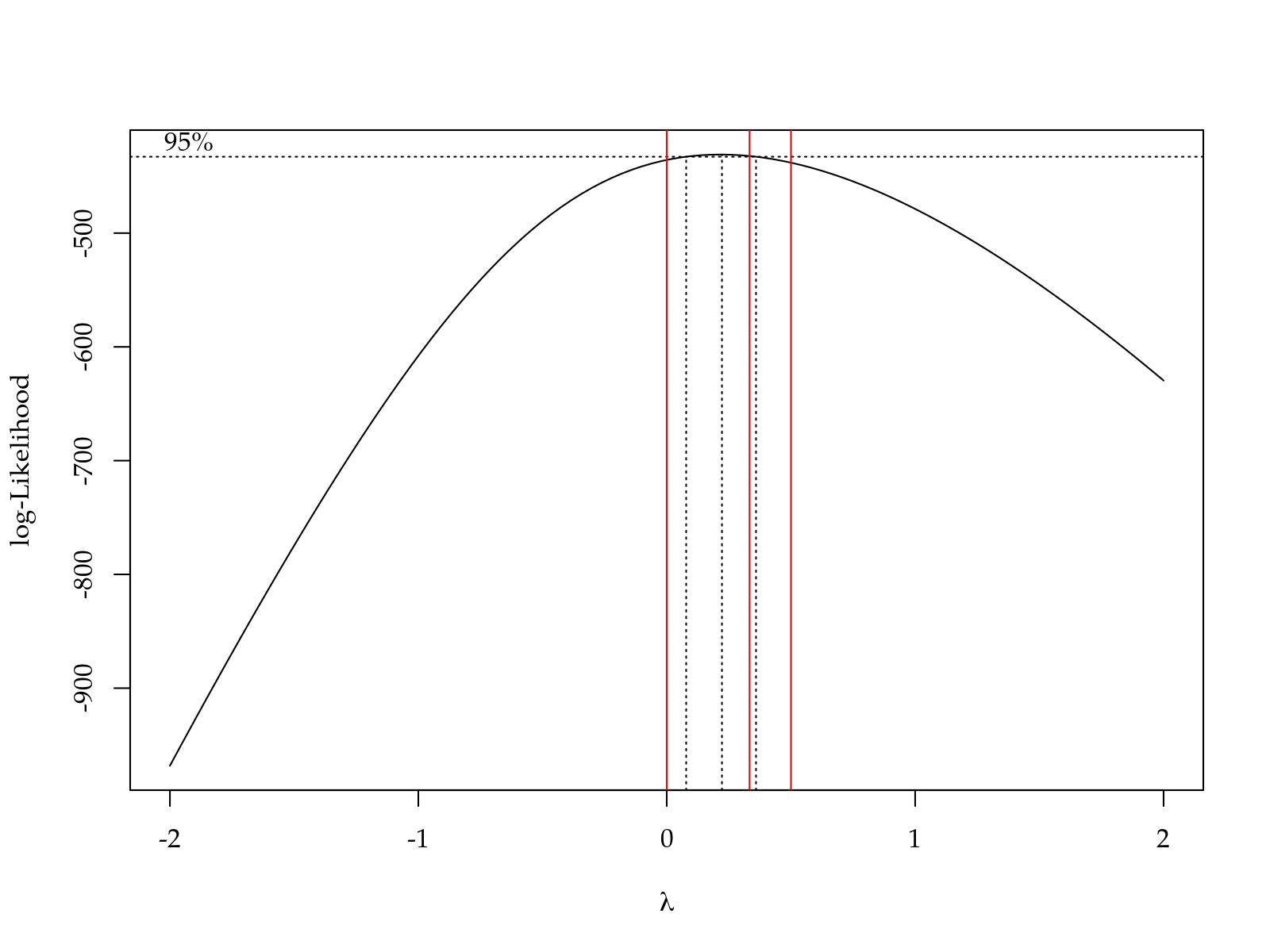
# Transformed variable.
da$y <- da$def^(1/3)

# Mixed models.
m0 <- lmer(y ~ yr/block + (yr + tra + hed)^2 + (1 | tre),
           data = da)

anova(m0)
## Type III Analysis of Variance Table with Satterthwaite's method
## Sum Sq Mean Sq NumDF DenDF F value Pr(>F)
## yr 7.0787 7.0787 1 168.149 20.0108 1.413e-05 ***
## tra 0.5304 0.1768 3 68.292 0.4998 0.683668
## hed 0.5451 0.5451 1 97.444 1.5409 0.217468
## yr:block 0.9078 0.4539 2 126.504 1.2832 0.280742
## yr:tra 1.6639 0.5546 3 140.721 1.5679 0.199874
## yr:hed 3.7688 3.7688 1 172.384 10.6540 0.001325 **
## tra:hed 0.3897 0.1299 3 99.179 0.3672 0.776836
## ---
## Signif. codes: 0 '***' 0.001 '**' 0.01 '*' 0.05 '.' 0.1 ' ' 1# summary(m0)# Fake model just to use the LE_matrix().
fake <- lm(nobars(formula(m0)), m0@frame)
cmp <- list()
# Main effect of fungicide.
L <- LE_matrix(fake, effect = "tra")
grid <- equallevels(attr(L, "grid"), da)
rownames(L) <- grid[, 1]
a <- apmc(X = L, model = m0, focus = "tra")
cmp$tra <- a
# Spliting the effect of head in each year.
L <- LE_matrix(fake, effect = c("yr", "hed"))
grid <- equallevels(attr(L, "grid"), da)
L <- by(L, grid$yr, as.matrix)
L <- lapply(L, "rownames<-", levels(grid$hed))
a <- ldply(lapply(L, apmc, model = m0, focus = "hed"), .id = "yr")
cmp$"yr:hed" <- ap1 <- segplot(tra ~ lwr + upr,
centers = fit,
data = cmp$tra,
draw = FALSE,
xlab = "Cubic root of defoliantion",
ylab = "Fungicides",
ann = sprintf("%0.2f %s",
cmp$tra$fit,
cmp$tra$cld)) +
layer(panel.text(x = centers[subscripts],
y = z[subscripts],
labels = ann[subscripts],
pos = 3))
p2 <- segplot(hed ~ lwr + upr | yr,
centers = fit,
data = cmp$"yr:hed",
draw = FALSE,
layout = c(1, NA),
xlab = "Cubic root of defoliantion",
ylab = "Hedging level",
as.table = TRUE,
ann = sprintf("%0.2f %s",
cmp$"yr:hed"$fit,
cmp$"yr:hed"$cld)) +
layer(panel.text(x = centers[subscripts],
y = z[subscripts],
labels = ann[subscripts],
pos = 3))
print(p1, position = c(0, 0.55, 1, 1), more = TRUE)
print(p2, position = c(0, 0, 1, 0.55))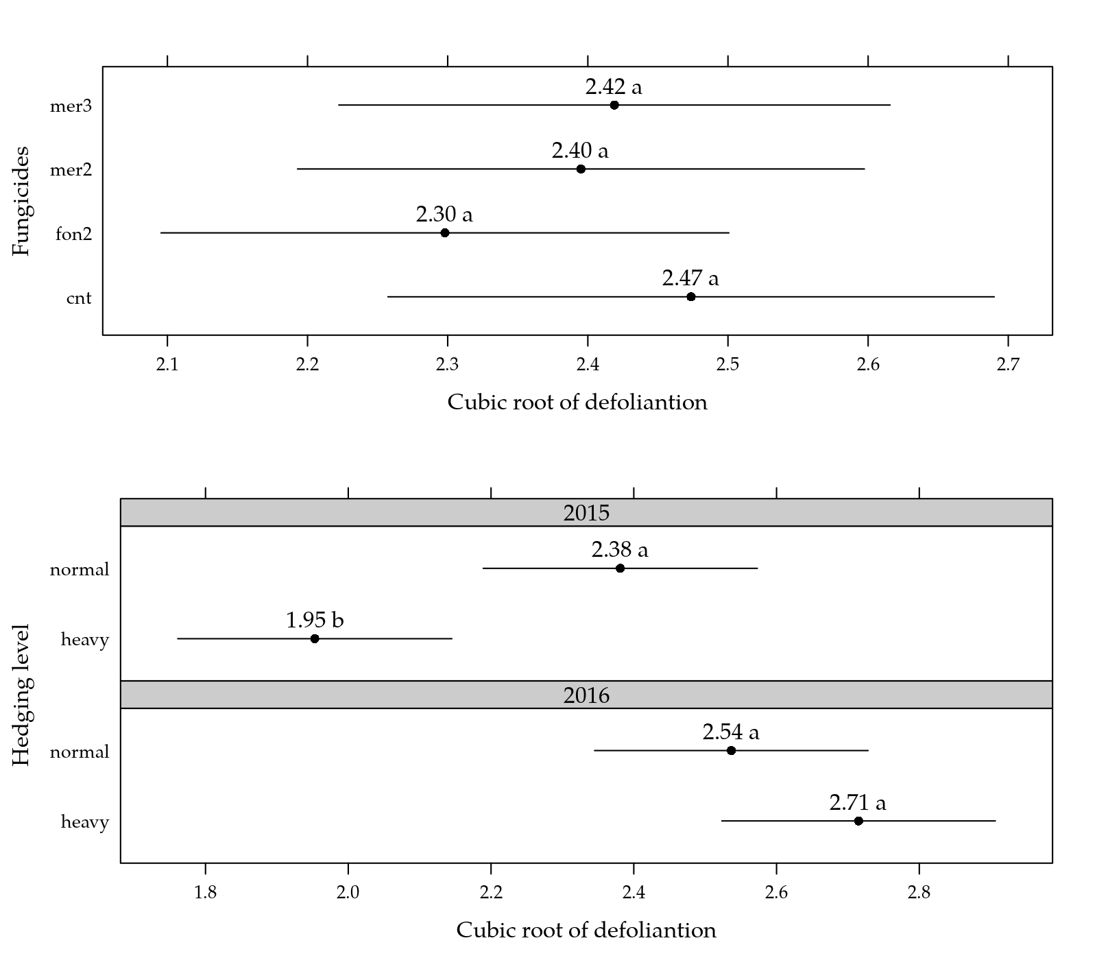
Figure 2: Cubic root means for defoliation as function of each factor levels.
Session information
## quinta, 11 de julho de 2019, 20:04
## ----------------------------------------
## R version 3.6.1 (2019-07-05)
## Platform: x86_64-pc-linux-gnu (64-bit)
## Running under: Ubuntu 18.04.2 LTS
##
## Matrix products: default
## BLAS:   /usr/lib/x86_64-linux-gnu/blas/libblas.so.3.7.1
## LAPACK: /usr/lib/x86_64-linux-gnu/lapack/liblapack.so.3.7.1
##
## locale:
##  [1] LC_CTYPE=pt_BR.UTF-8       LC_NUMERIC=C
##  [3] LC_TIME=pt_BR.UTF-8        LC_COLLATE=en_US.UTF-8
##  [5] LC_MONETARY=pt_BR.UTF-8    LC_MESSAGES=en_US.UTF-8
##  [7] LC_PAPER=pt_BR.UTF-8       LC_NAME=C
##  [9] LC_ADDRESS=C               LC_TELEPHONE=C
## [11] LC_MEASUREMENT=pt_BR.UTF-8 LC_IDENTIFICATION=C
##
## attached base packages:
## [1] stats     graphics  grDevices utils     datasets  methods
## [7] base
##
## other attached packages:
##  [1] captioner_2.2.3     knitr_1.23          RDASC_0.0-6
##  [4] wzRfun_0.81         lmerTest_3.1-0      lme4_1.1-21
##  [7] Matrix_1.2-17       multcomp_1.4-10     TH.data_1.0-10
## [10] MASS_7.3-51.4       survival_2.44-1.1   mvtnorm_1.0-11
## [13] doBy_4.6-2          reshape_0.8.8       plyr_1.8.4
## [16] latticeExtra_0.6-28 RColorBrewer_1.1-2  lattice_0.20-38
##
## loaded via a namespace (and not attached):
##  [1] zoo_1.8-6           tidyselect_0.2.5    xfun_0.8
##  [4] purrr_0.3.2         splines_3.6.1       tcltk_3.6.1
##  [7] colorspace_1.4-1    htmltools_0.3.6     rpanel_1.1-4
## [10] yaml_2.2.0          rlang_0.4.0         pkgdown_1.3.0
## [13] pillar_1.4.2        nloptr_1.2.1        glue_1.3.1
## [16] stringr_1.4.0       munsell_0.5.0       commonmark_1.7
## [19] gtable_0.3.0        codetools_0.2-16    memoise_1.1.0
## [22] evaluate_0.14       highr_0.8           Rcpp_1.0.1
## [25] backports_1.1.4     scales_1.0.0        desc_1.2.0
## [28] fs_1.3.1            ggplot2_3.2.0       digest_0.6.20
## [31] stringi_1.4.3       dplyr_0.8.3         numDeriv_2016.8-1.1
## [34] grid_3.6.1          rprojroot_1.3-2     tools_3.6.1
## [37] sandwich_2.5-1      magrittr_1.5        lazyeval_0.2.2
## [40] tibble_2.1.3        crayon_1.3.4        pkgconfig_2.0.2
## [43] xml2_1.2.0          assertthat_0.2.1    minqa_1.2.4
## [46] rmarkdown_1.13      roxygen2_6.1.1      R6_2.4.0
## [49] boot_1.3-23         nlme_3.1-140        compiler_3.6.1