Doses de Nitrogênio e Potássio para Cana-de-açúcar em Diferentes Sistemas de Manejo no Estado do Paraná
Walmes Zeviani & Michael Jonathan Fernandes Alves
2019-07-11
sugarcane_straw.RmdSession Definition
# https://github.com/walmes/wzRfun
# devtools::install_github("walmes/wzRfun")
library(wzRfun)

pks <- c("lattice",
         "gridExtra",
         "lme4",
         "lmerTest",
         "doBy",
         "multcomp")
sapply(pks, library, character.only = TRUE, logical.return = TRUE)library(RDASC)Exploratory data analysis
# Object structure.
str(sugarcane_straw)
## 'data.frame': 250 obs. of 11 variables:
## $ palha: int 1 1 1 1 1 1 1 1 1 1 ...
## $ bloc : int 1 2 3 4 5 1 2 3 4 5 ...
## $ K : int 0 0 0 0 0 0 0 0 0 0 ...
## $ N : int 0 0 0 0 0 45 45 45 45 45 ...
## $ ncm : num 6.26 6.47 7.98 8.6 7.48 7.14 7.66 7.99 7.31 7.68 ...
## $ pmc : num 1.05 1.22 1.26 1.2 1.2 1.39 1.14 1.26 1.3 1.29 ...
## $ tch : num 54.8 65.5 83.5 86 74.8 ...
## $ pol : num 14.7 15.2 14.9 15.6 16.1 ...
## $ tsh : num 8.02 9.99 12.45 13.45 12.01 ...
## $ tfn : num 17.3 17.3 18.1 18.9 15.8 ...
## $ tfk : num 16.8 18.6 14.7 15.9 15 ...## K 0 45 90 135 180
## palha N
## 1 0 5 5 5 5 5
## 45 5 5 5 5 5
## 90 5 5 5 5 5
## 135 5 5 5 5 5
## 180 5 5 5 5 5
## 2 0 5 5 5 5 5
## 45 5 5 5 5 5
## 90 5 5 5 5 5
## 135 5 5 5 5 5
## 180 5 5 5 5 5# Checking if is a complete cases dataset.
all(complete.cases(sugarcane_straw))## [1] TRUE# Descriptive measures.
summary(sugarcane_straw)## palha bloc K N
## Min. :1.0 Min. :1 Min. : 0 Min. : 0
## 1st Qu.:1.0 1st Qu.:2 1st Qu.: 45 1st Qu.: 45
## Median :1.5 Median :3 Median : 90 Median : 90
## Mean :1.5 Mean :3 Mean : 90 Mean : 90
## 3rd Qu.:2.0 3rd Qu.:4 3rd Qu.:135 3rd Qu.:135
## Max. :2.0 Max. :5 Max. :180 Max. :180
## ncm pmc tch pol
## Min. :5.150 Min. :0.780 Min. : 50.16 Min. :12.00
## 1st Qu.:7.665 1st Qu.:1.120 1st Qu.: 72.76 1st Qu.:14.90
## Median :7.970 Median :1.265 Median : 83.81 Median :15.20
## Mean :7.954 Mean :1.273 Mean : 84.62 Mean :15.25
## 3rd Qu.:8.287 3rd Qu.:1.438 3rd Qu.: 96.64 3rd Qu.:15.77
## Max. :9.720 Max. :1.640 Max. :128.36 Max. :17.90
## tsh tfn tfk
## Min. : 7.53 Min. : 7.65 Min. : 0.77
## 1st Qu.:10.89 1st Qu.:15.15 1st Qu.:14.37
## Median :12.93 Median :16.57 Median :15.62
## Mean :12.90 Mean :16.41 Mean :15.50
## 3rd Qu.:14.72 3rd Qu.:18.08 3rd Qu.:17.18
## Max. :21.44 Max. :21.33 Max. :20.13# A more detailed description.
# Hmisc::describe(sugarcane_straw)
# Create factors.
sugarcane_straw <- within(sugarcane_straw, {
# Convert integer to factor.
palha <- factor(sugarcane_straw$palha)
nit <- factor(sugarcane_straw$N)
pot <- factor(sugarcane_straw$K)
# Create a factor to represent main plots.
ue <- interaction(bloc, palha)
})Número de colmos por metro
#-----------------------------------------------------------------------
# To minimize modifications of code when analysing diferent responses.

# Define the legends for factors and variables.
leg <- list(N = expression("Nitrogênio"~(kg~ha^{-1})),
            K = expression("Potássio"~(kg~ha^{-1})),
            y = expression("Número de colmos por metro"),
            palha = c("Cobertura do solo", "Com palha", "Sem palha"))

# Use name y for the response.
sugarcane_straw$y <- sugarcane_straw$ncm

#-----------------------------------------------------------------------
# Scatter plots.

pk <- xyplot(y ~ K | palha, groups = N, data = sugarcane_straw,
             type = c("p", "a"),
             xlab = leg$K, ylab = leg$y,
             auto.key = list(title = leg$N,
                             cex.title = 1.1, columns = 5),
             strip = strip.custom(
                 strip.names = FALSE, strip.levels = TRUE,
                 factor.levels = c("Com palha", "Sem palha")))

pn <- xyplot(y ~ N | palha, groups = K, data = sugarcane_straw,
             type = c("p", "a"),
             xlab = leg$N, ylab = leg$y,
             auto.key = list(title = leg$K,
                             cex.title = 1.1, columns = 5),
             strip = strip.custom(
                 strip.names = FALSE, strip.levels = TRUE,
                 factor.levels = c("Com palha", "Sem palha")))

# grid.arrange(pn, pk)
# plot(pk)
plot(pn)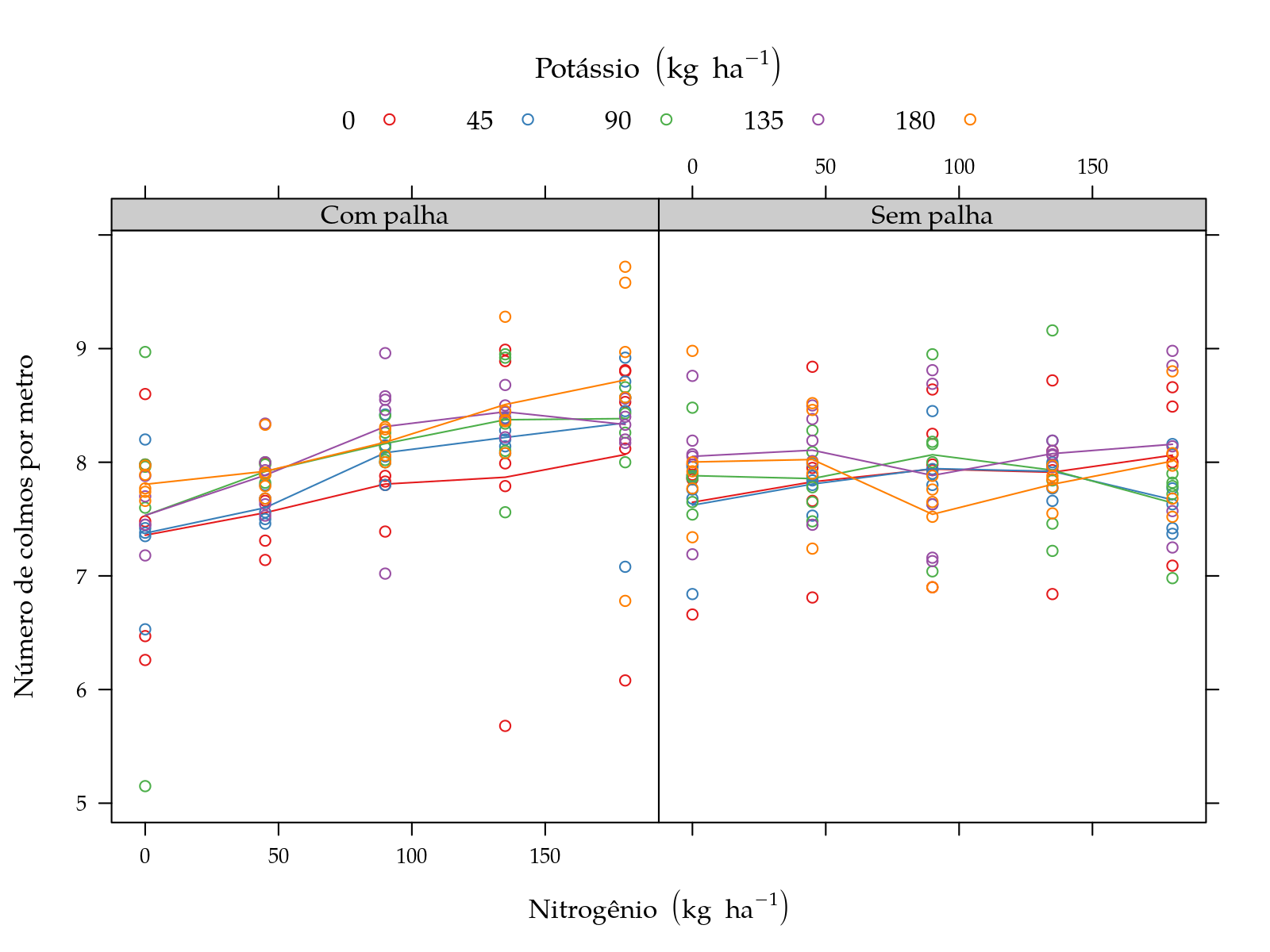
#-----------------------------------------------------------------------
# Model fitting.

# Saturated model.
m0 <- lmer(y ~ palha * nit * pot + (1 | bloc/ue),
           data = sugarcane_straw, REML = FALSE)

# Simple diagnostic.
plot(m0)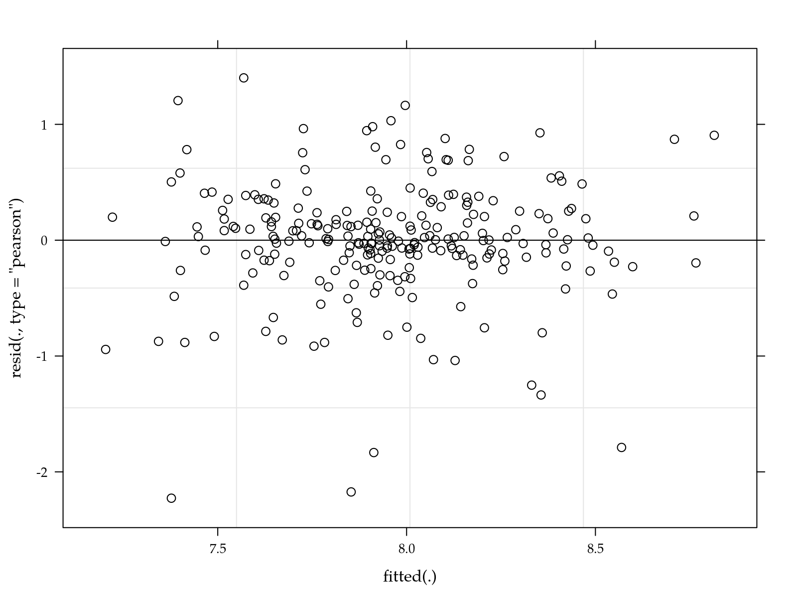
# qqnorm(residuals(m0, type = "pearson"))

# Estimates of the variance components.
VarCorr(m0)
## Groups Name Std.Dev.
## ue:bloc (Intercept) 0.072603
## bloc (Intercept) 0.085863
## Residual 0.508323# Tests for the fixed effects.
anova(m0)## Type III Analysis of Variance Table with Satterthwaite's method
## Sum Sq Mean Sq NumDF DenDF F value Pr(>F)
## palha 0.5593 0.55926 1 5 2.1644 0.2012070
## nit 7.2096 1.80240 4 240 6.9755 2.503e-05 ***
## pot 2.8398 0.70995 4 240 2.7476 0.0290209 *
## palha:nit 5.6340 1.40851 4 240 5.4511 0.0003231 ***
## palha:pot 1.6954 0.42385 4 240 1.6403 0.1647835
## nit:pot 1.6427 0.10267 16 240 0.3973 0.9823794
## palha:nit:pot 1.4598 0.09124 16 240 0.3531 0.9906184
## ---
## Signif. codes: 0 '***' 0.001 '**' 0.01 '*' 0.05 '.' 0.1 ' ' 1# Estimates of the effects and fitting measures.
# summary(m0)
# Drop non relevant terms.
# m1 <- update(m0, formula = . ~ palha * nit + pot + (1 | bloc/ue))
m1 <- lmer(y ~ palha * nit + pot + (1 | bloc/ue),
data = sugarcane_straw, REML = FALSE)
# Test the reduced model.
anova(m1, m0)## Data: sugarcane_straw
## Models:
## m1: y ~ palha * nit + pot + (1 | bloc/ue)
## m0: y ~ palha * nit * pot + (1 | bloc/ue)
## Df AIC BIC logLik deviance Chisq Chi Df Pr(>Chisq)
## m1 17 430.48 490.35 -198.24 396.48
## m0 53 484.60 671.23 -189.30 378.60 17.885 36 0.995anova(m1)## Type III Analysis of Variance Table with Satterthwaite's method
## Sum Sq Mean Sq NumDF DenDF F value Pr(>F)
## palha 0.6025 0.60251 1 5 2.1643 0.2012147
## nit 7.2096 1.80240 4 240 6.4745 5.793e-05 ***
## pot 2.8398 0.70995 4 240 2.5503 0.0398982 *
## palha:nit 5.6340 1.40851 4 240 5.0596 0.0006237 ***
## ---
## Signif. codes: 0 '***' 0.001 '**' 0.01 '*' 0.05 '.' 0.1 ' ' 1# summary(m1)
# Reducing by using linear effect for N and K.
m2 <- lmer(y ~ palha * N + K + (1 | bloc/ue),
data = sugarcane_straw, REML = FALSE)
# Test the reduced model.
anova(m2, m0)## Data: sugarcane_straw
## Models:
## m2: y ~ palha * N + K + (1 | bloc/ue)
## m0: y ~ palha * nit * pot + (1 | bloc/ue)
## Df AIC BIC logLik deviance Chisq Chi Df Pr(>Chisq)
## m2 8 415.76 443.93 -199.88 399.76
## m0 53 484.60 671.23 -189.30 378.60 21.162 45 0.9991anova(m2)## Type III Analysis of Variance Table with Satterthwaite's method
## Sum Sq Mean Sq NumDF DenDF F value Pr(>F)
## palha 1.6338 1.6338 1 28.724 5.7892 0.02279 *
## N 6.8750 6.8750 1 239.987 24.3603 1.495e-06 ***
## K 2.5461 2.5461 1 239.987 9.0218 0.00295 **
## palha:N 5.3437 5.3437 1 239.987 18.9346 2.002e-05 ***
## ---
## Signif. codes: 0 '***' 0.001 '**' 0.01 '*' 0.05 '.' 0.1 ' ' 1summary(m2)## Linear mixed model fit by maximum likelihood . t-tests use
## Satterthwaite's method [lmerModLmerTest]
## Formula: y ~ palha * N + K + (1 | bloc/ue)
## Data: sugarcane_straw
##
## AIC BIC logLik deviance df.resid
## 415.8 443.9 -199.9 399.8 242
##
## Scaled residuals:
## Min 1Q Median 3Q Max
## -4.5242 -0.4283 0.0610 0.4958 2.5748
##
## Random effects:
## Groups Name Variance Std.Dev.
## ue:bloc (Intercept) 0.004297 0.06556
## bloc (Intercept) 0.007379 0.08590
## Residual 0.282220 0.53124
## Number of obs: 250, groups: ue:bloc, 10; bloc, 5
##
## Fixed effects:
## Estimate Std. Error df t value Pr(>|t|)
## (Intercept) 7.428e+00 1.066e-01 5.131e+01 69.671 < 2e-16 ***
## palha2 2.973e-01 1.236e-01 2.872e+01 2.406 0.02279 *
## N 4.903e-03 7.466e-04 2.400e+02 6.567 3.15e-10 ***
## K 1.586e-03 5.280e-04 2.400e+02 3.004 0.00295 **
## palha2:N -4.595e-03 1.056e-03 2.400e+02 -4.351 2.00e-05 ***
## ---
## Signif. codes: 0 '***' 0.001 '**' 0.01 '*' 0.05 '.' 0.1 ' ' 1
##
## Correlation of Fixed Effects:
## (Intr) palha2 N K
## palha2 -0.579
## N -0.630 0.544
## K -0.446 0.000 0.000
## palha2:N 0.446 -0.769 -0.707 0.000
## convergence code: 0
## Model failed to converge with max|grad| = 0.00268305 (tol = 0.002, component 1)# Final model.
mod <- m2
#-----------------------------------------------------------------------
# Fitted values.
# Experimental values to get estimates.
grid <- with(sugarcane_straw,
expand.grid(palha = levels(palha),
N = seq(min(N), max(N), length.out = 10),
K = seq(min(N), max(N), length.out = 3),
KEEP.OUT.ATTRS = FALSE))
# Matrix of fixed effects.
X <- model.matrix(terms(mod), data = cbind(grid, y = 0))
# Confidence intervals.
ci <- confint(glht(mod, linfct = X),
calpha = univariate_calpha())$confint
colnames(ci)[1] <- "fit"
grid <- cbind(grid, ci)
str(grid)## 'data.frame': 60 obs. of 6 variables:
## $ palha: Factor w/ 2 levels "1","2": 1 2 1 2 1 2 1 2 1 2 ...
## $ N : num 0 0 20 20 40 40 60 60 80 80 ...
## $ K : num 0 0 0 0 0 0 0 0 0 0 ...
## $ fit : num 7.43 7.73 7.53 7.73 7.62 ...
## $ lwr : num 7.22 7.52 7.33 7.54 7.45 ...
## $ upr : num 7.64 7.93 7.72 7.92 7.8 ...# Sample averages.
# averages <- aggregate(nobars(formula(mod)),
# data = sugarcane_straw, FUN = mean)
#
# xyplot(y ~ N | factor(K), groups = palha, data = averages,
# type = "o", as.table = TRUE)
xyplot(fit ~ N | factor(K), groups = palha, data = grid,
type = "l", as.table = TRUE, layout = c(NA, 1),
xlab = leg$N, ylab = leg$y,
auto.key = list(title = leg$palha[1], cex.title = 1.1,
text = c(leg$palha[-1]), columns = 2,
points = FALSE, lines = TRUE),
uy = grid$upr, ly = grid$lwr,
cty = "bands", alpha = 0.25, fill = "gray50",
prepanel = prepanel.cbH,
panel.groups = panel.cbH,
panel = panel.superpose)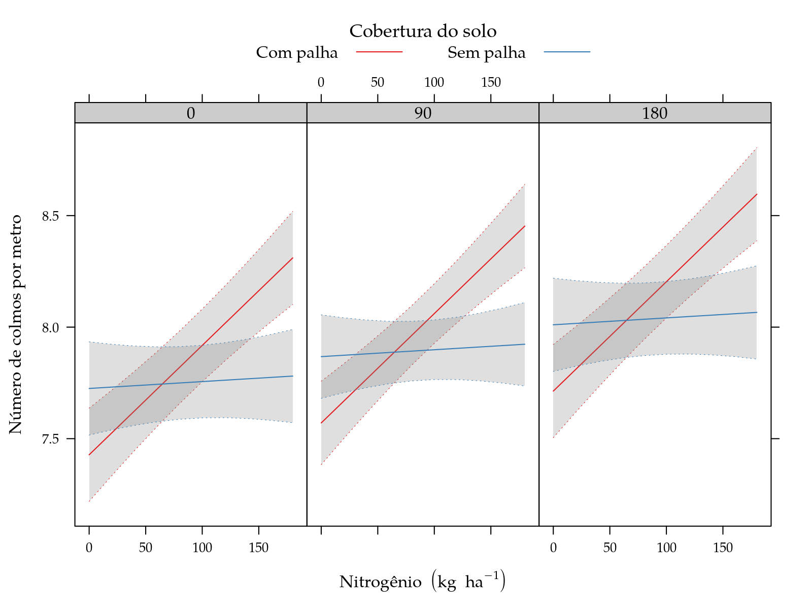
Peso médio de colmo
#-----------------------------------------------------------------------

leg$y <- "Peso médio de colmo (kg)"
sugarcane_straw$y <- sugarcane_straw$pmc

#-----------------------------------------------------------------------
# Scatter plots.

pk <- xyplot(y ~ K | palha, groups = N, data = sugarcane_straw,
             type = c("p", "a"),
             xlab = leg$K, ylab = leg$y,
             auto.key = list(title = leg$N,
                             cex.title = 1.1, columns = 5),
             strip = strip.custom(
                 strip.names = FALSE, strip.levels = TRUE,
                 factor.levels = c("Com palha", "Sem palha")))

pn <- xyplot(y ~ N | palha, groups = K, data = sugarcane_straw,
             type = c("p", "a"),
             xlab = leg$N, ylab = leg$y,
             auto.key = list(title = leg$K,
                             cex.title = 1.1, columns = 5),
             strip = strip.custom(
                 strip.names = FALSE, strip.levels = TRUE,
                 factor.levels = c("Com palha", "Sem palha")))

# grid.arrange(pn, pk)
# plot(pk)
plot(pn)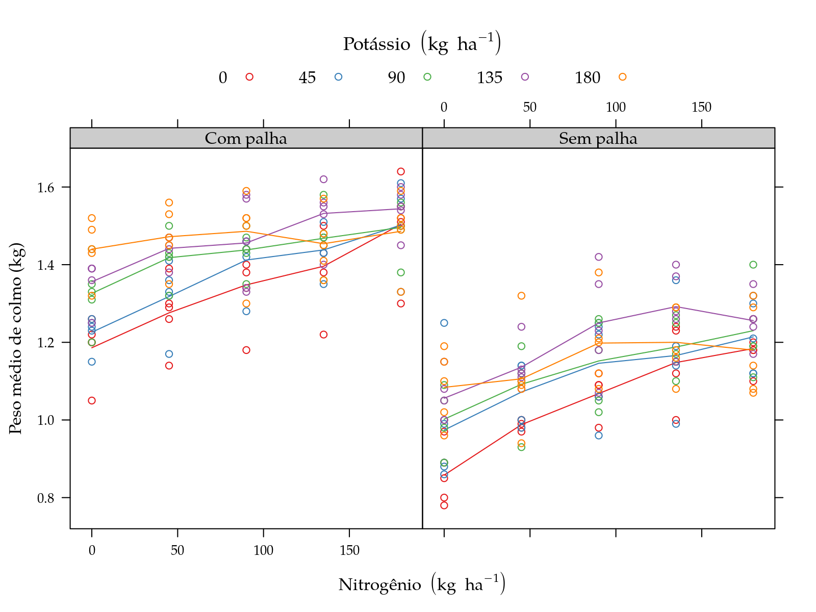
#-----------------------------------------------------------------------
# Model fitting.

# Saturated model.
m0 <- lmer(y ~ palha * nit * pot + (1 | bloc/ue),
           data = sugarcane_straw, REML = FALSE)

# Simple diagnostic.
plot(m0)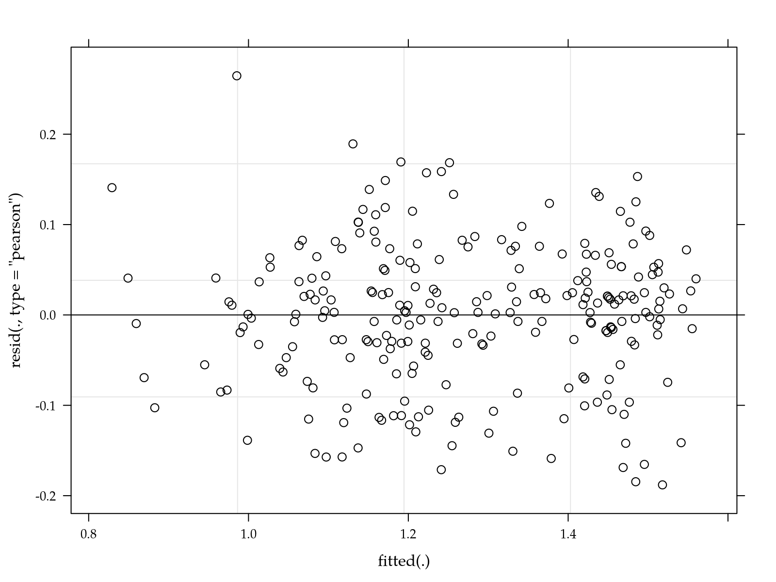
# qqnorm(residuals(m0, type = "pearson"))

# Estimates of the variance components.
VarCorr(m0)
## Groups Name Std.Dev.
## ue:bloc (Intercept) 0.0203030
## bloc (Intercept) 0.0052569
## Residual 0.0795325# Tests for the fixed effects.
anova(m0)## Type III Analysis of Variance Table with Satterthwaite's method
## Sum Sq Mean Sq NumDF DenDF F value Pr(>F)
## palha 1.96077 1.96077 1 5.008 309.9831 1.069e-05 ***
## nit 1.38310 0.34577 4 240.000 54.6644 < 2.2e-16 ***
## pot 0.58179 0.14545 4 240.000 22.9941 4.238e-16 ***
## palha:nit 0.02894 0.00724 4 240.000 1.1438 0.336549
## palha:pot 0.02131 0.00533 4 240.000 0.8422 0.499623
## nit:pot 0.21837 0.01365 16 240.000 2.1577 0.006996 **
## palha:nit:pot 0.03237 0.00202 16 240.000 0.3199 0.994604
## ---
## Signif. codes: 0 '***' 0.001 '**' 0.01 '*' 0.05 '.' 0.1 ' ' 1# Estimates of the effects and fitting measures.
# summary(m0)
# Drop non relevant terms.
# m1 <- update(m0, formula = . ~ palha * nit + pot + (1 | bloc/ue))
m1 <- lmer(y ~ palha + nit * pot + (1 | bloc/ue),
data = sugarcane_straw, REML = FALSE)
# Test the reduced model.
anova(m1, m0)## Data: sugarcane_straw
## Models:
## m1: y ~ palha + nit * pot + (1 | bloc/ue)
## m0: y ~ palha * nit * pot + (1 | bloc/ue)
## Df AIC BIC logLik deviance Chisq Chi Df Pr(>Chisq)
## m1 29 -475.54 -373.42 266.77 -533.54
## m0 53 -440.26 -253.62 273.13 -546.26 12.719 24 0.9705anova(m1)## Type III Analysis of Variance Table with Satterthwaite's method
## Sum Sq Mean Sq NumDF DenDF F value Pr(>F)
## palha 2.06539 2.06539 1 4.997 309.6743 1.092e-05 ***
## nit 1.38310 0.34577 4 240.003 51.8438 < 2.2e-16 ***
## pot 0.58179 0.14545 4 240.003 21.8076 2.297e-15 ***
## nit:pot 0.21837 0.01365 16 240.003 2.0464 0.01136 *
## ---
## Signif. codes: 0 '***' 0.001 '**' 0.01 '*' 0.05 '.' 0.1 ' ' 1# summary(m1)
# Reducing by using linear effect for N and K.
m2 <- lmer(y ~ palha + N * K + (1 | bloc/ue),
data = sugarcane_straw, REML = FALSE)
# Test the reduced model.
anova(m2, m0)## Data: sugarcane_straw
## Models:
## m2: y ~ palha + N * K + (1 | bloc/ue)
## m0: y ~ palha * nit * pot + (1 | bloc/ue)
## Df AIC BIC logLik deviance Chisq Chi Df Pr(>Chisq)
## m2 8 -490.31 -462.14 253.16 -506.31
## m0 53 -440.26 -253.62 273.13 -546.26 39.948 45 0.6854anova(m2)## Type III Analysis of Variance Table with Satterthwaite's method
## Sum Sq Mean Sq NumDF DenDF F value Pr(>F)
## palha 2.31509 2.31509 1 5.008 309.881 1.071e-05 ***
## N 1.00829 1.00829 1 240.001 134.962 < 2.2e-16 ***
## K 0.55912 0.55912 1 240.001 74.840 7.454e-16 ***
## N:K 0.17424 0.17424 1 240.001 23.323 2.442e-06 ***
## ---
## Signif. codes: 0 '***' 0.001 '**' 0.01 '*' 0.05 '.' 0.1 ' ' 1summary(m2)## Linear mixed model fit by maximum likelihood . t-tests use
## Satterthwaite's method [lmerModLmerTest]
## Formula: y ~ palha + N * K + (1 | bloc/ue)
## Data: sugarcane_straw
##
## AIC BIC logLik deviance df.resid
## -490.3 -462.1 253.2 -506.3 242
##
## Scaled residuals:
## Min 1Q Median 3Q Max
## -2.54434 -0.53260 0.04472 0.63706 3.13341
##
## Random effects:
## Groups Name Variance Std.Dev.
## ue:bloc (Intercept) 3.666e-04 0.019147
## bloc (Intercept) 2.754e-05 0.005248
## Residual 7.471e-03 0.086434
## Number of obs: 250, groups: ue:bloc, 10; bloc, 5
##
## Fixed effects:
## Estimate Std. Error df t value Pr(>|t|)
## (Intercept) 1.198e+00 1.943e-02 6.596e+01 61.656 < 2e-16 ***
## palha2 -2.872e-01 1.631e-02 5.008e+00 -17.603 1.07e-05 ***
## N 1.728e-03 1.488e-04 2.400e+02 11.617 < 2e-16 ***
## K 1.287e-03 1.488e-04 2.400e+02 8.651 7.45e-16 ***
## N:K -6.519e-06 1.350e-06 2.400e+02 -4.829 2.44e-06 ***
## ---
## Signif. codes: 0 '***' 0.001 '**' 0.01 '*' 0.05 '.' 0.1 ' ' 1
##
## Correlation of Fixed Effects:
## (Intr) palha2 N K
## palha2 -0.420
## N -0.689 0.000
## K -0.689 0.000 0.667
## N:K 0.563 0.000 -0.816 -0.816
## fit warnings:
## Some predictor variables are on very different scales: consider rescaling# Final model.
mod <- m2
#-----------------------------------------------------------------------
# Fitted values.
# Experimental values to get estimates.
grid <- with(sugarcane_straw,
expand.grid(palha = levels(palha),
N = seq(min(N), max(N), length.out = 10),
K = seq(min(N), max(N), length.out = 3),
KEEP.OUT.ATTRS = FALSE))
# Matrix of fixed effects.
X <- model.matrix(terms(mod), data = cbind(grid, y = 0))
# Confidence intervals.
ci <- confint(glht(mod, linfct = X),
calpha = univariate_calpha())$confint
colnames(ci)[1] <- "fit"
grid <- cbind(grid, ci)
str(grid)## 'data.frame': 60 obs. of 6 variables:
## $ palha: Factor w/ 2 levels "1","2": 1 2 1 2 1 2 1 2 1 2 ...
## $ N : num 0 0 20 20 40 40 60 60 80 80 ...
## $ K : num 0 0 0 0 0 0 0 0 0 0 ...
## $ fit : num 1.198 0.911 1.233 0.946 1.267 ...
## $ lwr : num 1.16 0.873 1.198 0.911 1.236 ...
## $ upr : num 1.236 0.949 1.267 0.98 1.299 ...# Sample averages.
# averages <- aggregate(nobars(formula(mod)),
# data = sugarcane_straw, FUN = mean)
#
# xyplot(y ~ N | factor(K), groups = palha, data = averages,
# type = "o", as.table = TRUE)
xyplot(fit ~ N | factor(K), groups = palha, data = grid,
type = "l", as.table = TRUE, layout = c(NA, 1),
xlab = leg$N, ylab = leg$y,
auto.key = list(title = leg$palha[1], cex.title = 1.1,
text = c(leg$palha[-1]), columns = 2,
points = FALSE, lines = TRUE),
uy = grid$upr, ly = grid$lwr,
cty = "bands", alpha = 0.25, fill = "gray50",
prepanel = prepanel.cbH,
panel.groups = panel.cbH,
panel = panel.superpose)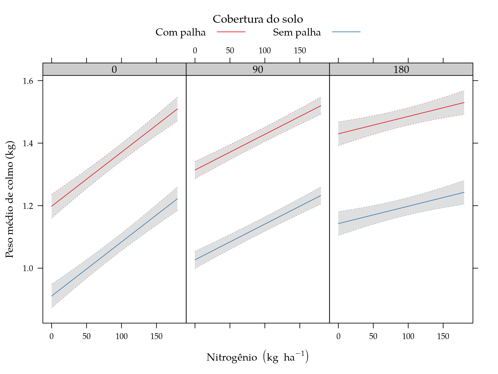
Produção de cana-de-açúcar
#-----------------------------------------------------------------------

leg$y <- expression("Produção de cana"~(ton~ha^{-1}))
sugarcane_straw$y <- sugarcane_straw$tch

#-----------------------------------------------------------------------
# Scatter plots.

pk <- xyplot(y ~ K | palha, groups = N, data = sugarcane_straw,
             type = c("p", "a"),
             xlab = leg$K, ylab = leg$y,
             auto.key = list(title = leg$N,
                             cex.title = 1.1, columns = 5),
             strip = strip.custom(
                 strip.names = FALSE, strip.levels = TRUE,
                 factor.levels = c("Com palha", "Sem palha")))

pn <- xyplot(y ~ N | palha, groups = K, data = sugarcane_straw,
             type = c("p", "a"),
             xlab = leg$N, ylab = leg$y,
             auto.key = list(title = leg$K,
                             cex.title = 1.1, columns = 5),
             strip = strip.custom(
                 strip.names = FALSE, strip.levels = TRUE,
                 factor.levels = c("Com palha", "Sem palha")))

# grid.arrange(pn, pk)
# plot(pk)
plot(pn)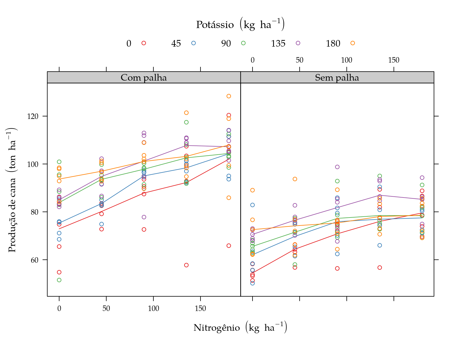
#-----------------------------------------------------------------------
# Model fitting.

# Saturated model.
m0 <- lmer(y ~ palha * nit * pot + (1 | bloc/ue),
           data = sugarcane_straw, REML = FALSE)

# Simple diagnostic.
plot(m0)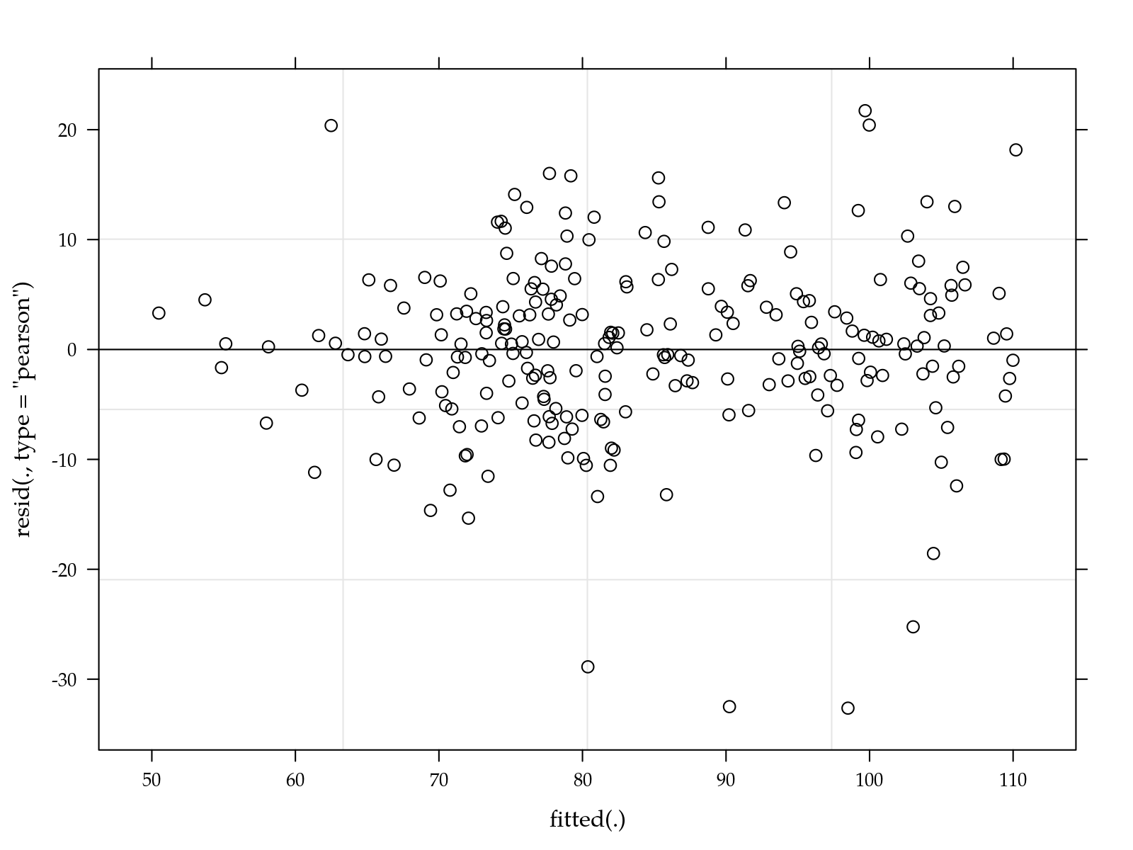
# qqnorm(residuals(m0, type = "pearson"))

# Estimates of the variance components.
VarCorr(m0)
## Groups Name Std.Dev.
## ue:bloc (Intercept) 2.4203
## bloc (Intercept) 1.2705
## Residual 7.9437# Tests for the fixed effects.
anova(m0)## Type III Analysis of Variance Table with Satterthwaite's method
## Sum Sq Mean Sq NumDF DenDF F value Pr(>F)
## palha 7969.9 7969.9 1 5.001 126.3007 9.733e-05 ***
## nit 11639.3 2909.8 4 240.002 46.1122 < 2.2e-16 ***
## pot 4494.9 1123.7 4 240.002 17.8079 8.121e-13 ***
## palha:nit 494.8 123.7 4 240.002 1.9603 0.1013
## palha:pot 411.0 102.8 4 240.002 1.6283 0.1678
## nit:pot 1195.5 74.7 16 240.002 1.1841 0.2813
## palha:nit:pot 168.3 10.5 16 240.002 0.1667 0.9999
## ---
## Signif. codes: 0 '***' 0.001 '**' 0.01 '*' 0.05 '.' 0.1 ' ' 1# Estimates of the effects and fitting measures.
# summary(m0)
# Drop non relevant terms.
# m1 <- update(m0, formula = . ~ palha * nit + pot + (1 | bloc/ue))
m1 <- lmer(y ~ palha + nit + pot + (1 | bloc/ue),
data = sugarcane_straw, REML = FALSE)
# Test the reduced model.
anova(m1, m0)## Data: sugarcane_straw
## Models:
## m1: y ~ palha + nit + pot + (1 | bloc/ue)
## m0: y ~ palha * nit * pot + (1 | bloc/ue)
## Df AIC BIC logLik deviance Chisq Chi Df Pr(>Chisq)
## m1 13 1818.8 1864.6 -896.40 1792.8
## m0 53 1865.3 2051.9 -879.65 1759.3 33.514 40 0.7558anova(m1)## Type III Analysis of Variance Table with Satterthwaite's method
## Sum Sq Mean Sq NumDF DenDF F value Pr(>F)
## palha 9165.9 9165.9 1 5 126.321 9.741e-05 ***
## nit 11639.3 2909.8 4 240 40.102 < 2.2e-16 ***
## pot 4494.9 1123.7 4 240 15.487 2.768e-11 ***
## ---
## Signif. codes: 0 '***' 0.001 '**' 0.01 '*' 0.05 '.' 0.1 ' ' 1# summary(m1)
# Reducing by using linear effect for N and K.
m2 <- lmer(y ~ palha + N + K + (1 | bloc/ue),
data = sugarcane_straw, REML = FALSE)
# Test the reduced model.
anova(m2, m0)## Data: sugarcane_straw
## Models:
## m2: y ~ palha + N + K + (1 | bloc/ue)
## m0: y ~ palha * nit * pot + (1 | bloc/ue)
## Df AIC BIC logLik deviance Chisq Chi Df Pr(>Chisq)
## m2 7 1820.2 1844.9 -903.11 1806.2
## m0 53 1865.3 2051.9 -879.65 1759.3 46.932 46 0.4341anova(m2)## Type III Analysis of Variance Table with Satterthwaite's method
## Sum Sq Mean Sq NumDF DenDF F value Pr(>F)
## palha 9694.5 9694.5 1 5 126.34 9.730e-05 ***
## N 11187.3 11187.3 1 240 145.80 < 2.2e-16 ***
## K 3945.6 3945.6 1 240 51.42 9.187e-12 ***
## ---
## Signif. codes: 0 '***' 0.001 '**' 0.01 '*' 0.05 '.' 0.1 ' ' 1summary(m2)## Linear mixed model fit by maximum likelihood . t-tests use
## Satterthwaite's method [lmerModLmerTest]
## Formula: y ~ palha + N + K + (1 | bloc/ue)
## Data: sugarcane_straw
##
## AIC BIC logLik deviance df.resid
## 1820.2 1844.9 -903.1 1806.2 243
##
## Scaled residuals:
## Min 1Q Median 3Q Max
## -3.9369 -0.5248 0.0271 0.6189 2.6763
##
## Random effects:
## Groups Name Variance Std.Dev.
## ue:bloc (Intercept) 5.310 2.304
## bloc (Intercept) 1.614 1.270
## Residual 76.733 8.760
## Number of obs: 250, groups: ue:bloc, 10; bloc, 5
##
## Fixed effects:
## Estimate Std. Error df t value Pr(>|t|)
## (Intercept) 79.830440 1.796206 25.015330 44.444 < 2e-16 ***
## palha2 -20.578400 1.830797 5.000354 -11.240 9.73e-05 ***
## N 0.105115 0.008705 239.999500 12.075 < 2e-16 ***
## K 0.062425 0.008705 239.999500 7.171 9.19e-12 ***
## ---
## Signif. codes: 0 '***' 0.001 '**' 0.01 '*' 0.05 '.' 0.1 ' ' 1
##
## Correlation of Fixed Effects:
## (Intr) palha2 N
## palha2 -0.510
## N -0.436 0.000
## K -0.436 0.000 0.000# Final model.
mod <- m2
#-----------------------------------------------------------------------
# Fitted values.
# Experimental values to get estimates.
grid <- with(sugarcane_straw,
expand.grid(palha = levels(palha),
N = seq(min(N), max(N), length.out = 10),
K = seq(min(N), max(N), length.out = 3),
KEEP.OUT.ATTRS = FALSE))
# Matrix of fixed effects.
X <- model.matrix(terms(mod), data = cbind(grid, y = 0))
# Confidence intervals.
ci <- confint(glht(mod, linfct = X),
calpha = univariate_calpha())$confint
colnames(ci)[1] <- "fit"
grid <- cbind(grid, ci)
str(grid)## 'data.frame': 60 obs. of 6 variables:
## $ palha: Factor w/ 2 levels "1","2": 1 2 1 2 1 2 1 2 1 2 ...
## $ N : num 0 0 20 20 40 40 60 60 80 80 ...
## $ K : num 0 0 0 0 0 0 0 0 0 0 ...
## $ fit : num 79.8 59.3 81.9 61.4 84 ...
## $ lwr : num 76.3 55.7 78.5 58 80.8 ...
## $ upr : num 83.4 62.8 85.3 64.7 87.3 ...# Sample averages.
# averages <- aggregate(nobars(formula(mod)),
# data = sugarcane_straw, FUN = mean)
#
# xyplot(y ~ N | factor(K), groups = palha, data = averages,
# type = "o", as.table = TRUE)
xyplot(fit ~ N | factor(K), groups = palha, data = grid,
type = "l", as.table = TRUE, layout = c(NA, 1),
xlab = leg$N, ylab = leg$y,
auto.key = list(title = leg$palha[1], cex.title = 1.1,
text = c(leg$palha[-1]), columns = 2,
points = FALSE, lines = TRUE),
uy = grid$upr, ly = grid$lwr,
cty = "bands", alpha = 0.25, fill = "gray50",
prepanel = prepanel.cbH,
panel.groups = panel.cbH,
panel = panel.superpose)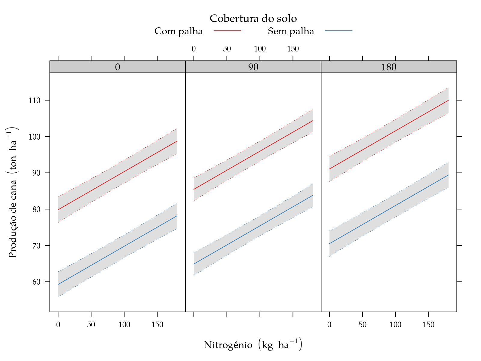
Teor de sacarose aparente
#-----------------------------------------------------------------------

leg$y <- "Teor de sacarose aparente"
sugarcane_straw$y <- sugarcane_straw$pol

#-----------------------------------------------------------------------
# Scatter plots.

pk <- xyplot(y ~ K | palha, groups = N, data = sugarcane_straw,
             type = c("p", "a"),
             xlab = leg$K, ylab = leg$y,
             auto.key = list(title = leg$N,
                             cex.title = 1.1, columns = 5),
             strip = strip.custom(
                 strip.names = FALSE, strip.levels = TRUE,
                 factor.levels = c("Com palha", "Sem palha")))

pn <- xyplot(y ~ N | palha, groups = K, data = sugarcane_straw,
             type = c("p", "a"),
             xlab = leg$N, ylab = leg$y,
             auto.key = list(title = leg$K,
                             cex.title = 1.1, columns = 5),
             strip = strip.custom(
                 strip.names = FALSE, strip.levels = TRUE,
                 factor.levels = c("Com palha", "Sem palha")))

# grid.arrange(pn, pk)
# plot(pk)
plot(pn)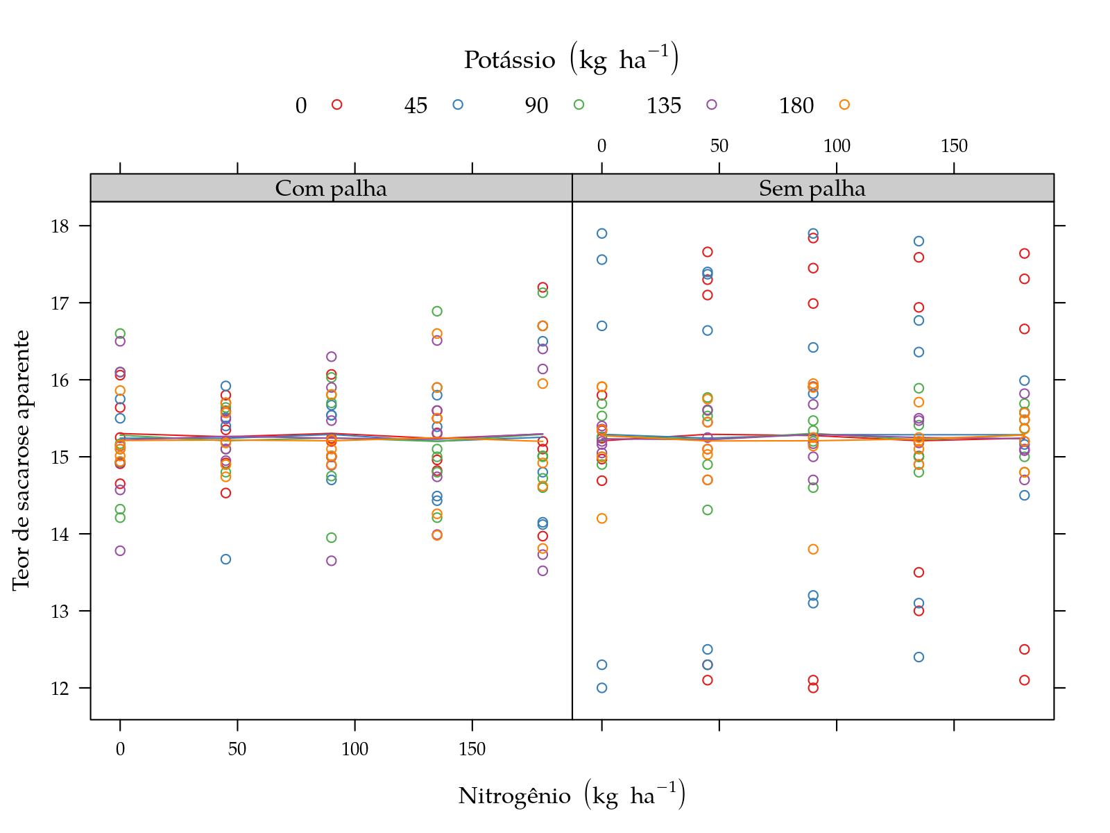
#-----------------------------------------------------------------------
# Model fitting.

# Saturated model.
m0 <- lmer(y ~ palha * nit * pot + (1 | bloc/ue),
           data = sugarcane_straw, REML = FALSE)

# Simple diagnostic.
plot(m0)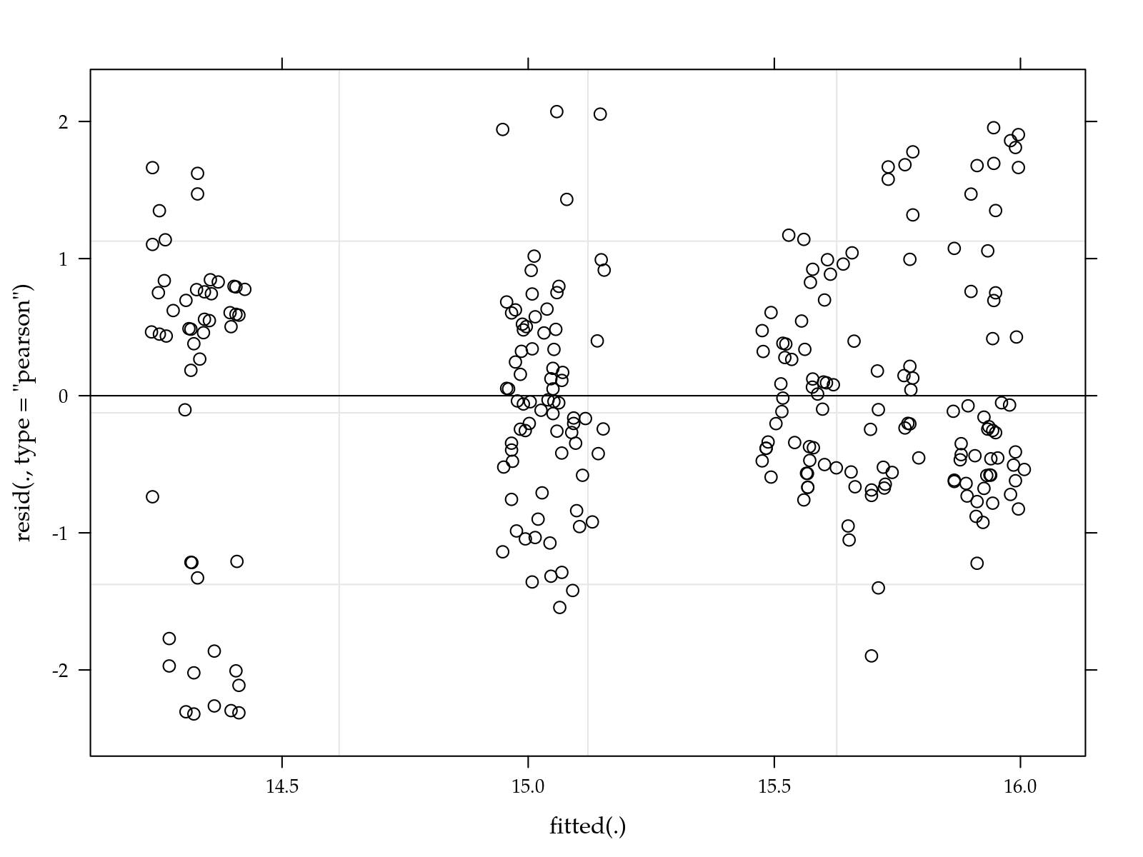
# qqnorm(residuals(m0, type = "pearson"))

# Estimates of the variance components.
VarCorr(m0)
## Groups Name Std.Dev.
## ue:bloc (Intercept) 0.59515
## bloc (Intercept) 0.00000
## Residual 0.92467# Tests for the fixed effects.
anova(m0)## Type III Analysis of Variance Table with Satterthwaite's method
## Sum Sq Mean Sq NumDF DenDF F value Pr(>F)
## palha 0.000261 0.0002605 1 10 0.0003 0.9864
## nit 0.053042 0.0132606 4 240 0.0155 0.9995
## pot 0.038214 0.0095536 4 240 0.0112 0.9998
## palha:nit 0.003798 0.0009494 4 240 0.0011 1.0000
## palha:pot 0.036210 0.0090524 4 240 0.0106 0.9998
## nit:pot 0.070650 0.0044156 16 240 0.0052 1.0000
## palha:nit:pot 0.079654 0.0049784 16 240 0.0058 1.0000# Estimates of the effects and fitting measures.
# summary(m0)Produção de sacarose
#-----------------------------------------------------------------------

leg$y <- expression("Sacarose"~(ton~ha^{-1}))
sugarcane_straw$y <- sugarcane_straw$tsh

#-----------------------------------------------------------------------
# Scatter plots.

pk <- xyplot(y ~ K | palha, groups = N, data = sugarcane_straw,
             type = c("p", "a"),
             xlab = leg$K, ylab = leg$y,
             auto.key = list(title = leg$N,
                             cex.title = 1.1, columns = 5),
             strip = strip.custom(
                 strip.names = FALSE, strip.levels = TRUE,
                 factor.levels = c("Com palha", "Sem palha")))

pn <- xyplot(y ~ N | palha, groups = K, data = sugarcane_straw,
             type = c("p", "a"),
             xlab = leg$N, ylab = leg$y,
             auto.key = list(title = leg$K,
                             cex.title = 1.1, columns = 5),
             strip = strip.custom(
                 strip.names = FALSE, strip.levels = TRUE,
                 factor.levels = c("Com palha", "Sem palha")))

# grid.arrange(pn, pk)
# plot(pk)
plot(pn)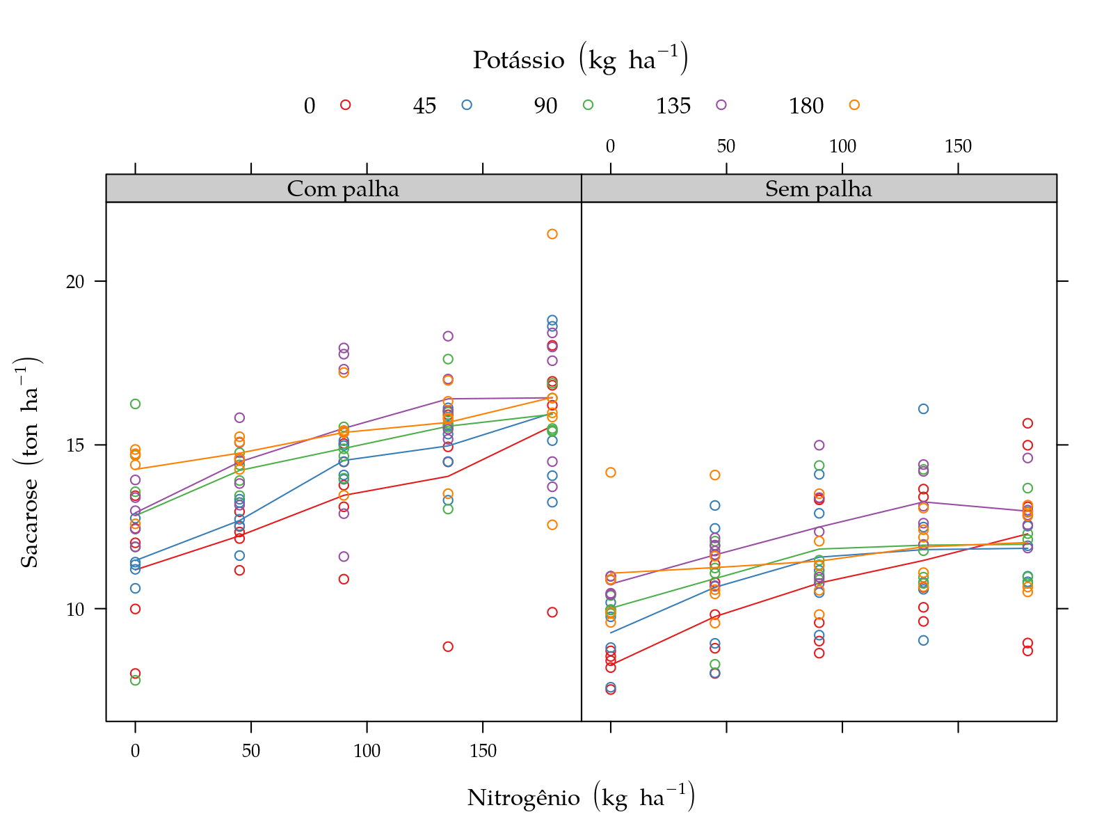
#-----------------------------------------------------------------------
# Model fitting.

# Saturated model.
m0 <- lmer(y ~ palha * nit * pot + (1 | bloc/ue),
           data = sugarcane_straw, REML = FALSE)

# Simple diagnostic.
plot(m0)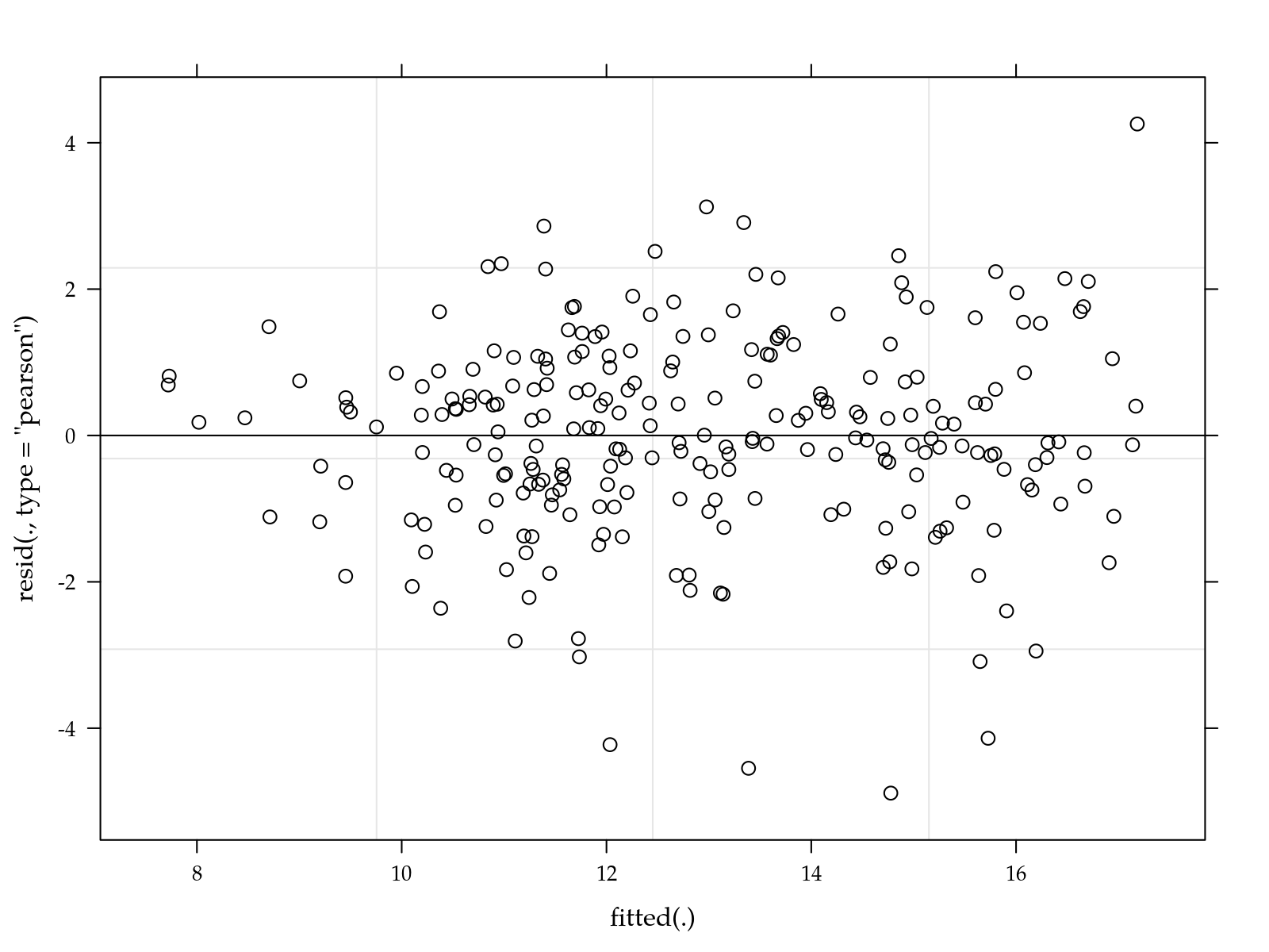
# qqnorm(residuals(m0, type = "pearson"))

# Estimates of the variance components.
VarCorr(m0)
## Groups Name Std.Dev.
## ue:bloc (Intercept) 0.68218
## bloc (Intercept) 0.00000
## Residual 1.37393# Tests for the fixed effects.
anova(m0)## Type III Analysis of Variance Table with Satterthwaite's method
## Sum Sq Mean Sq NumDF DenDF F value Pr(>F)
## palha 86.426 86.426 1 10 45.7840 4.941e-05 ***
## nit 278.180 69.545 4 240 36.8414 < 2.2e-16 ***
## pot 103.586 25.896 4 240 13.7186 4.334e-10 ***
## palha:nit 10.766 2.692 4 240 1.4259 0.2260
## palha:pot 8.375 2.094 4 240 1.1091 0.3528
## nit:pot 29.942 1.871 16 240 0.9913 0.4668
## palha:nit:pot 3.930 0.246 16 240 0.1301 1.0000
## ---
## Signif. codes: 0 '***' 0.001 '**' 0.01 '*' 0.05 '.' 0.1 ' ' 1# Estimates of the effects and fitting measures.
# summary(m0)
# Drop non relevant terms.
# m1 <- update(m0, formula = . ~ palha * nit + pot + (1 | bloc/ue))
m1 <- lmer(y ~ palha + nit + pot + (1 | bloc/ue),
data = sugarcane_straw, REML = FALSE)
# Test the reduced model.
anova(m1, m0)## Data: sugarcane_straw
## Models:
## m1: y ~ palha + nit + pot + (1 | bloc/ue)
## m0: y ~ palha * nit * pot + (1 | bloc/ue)
## Df AIC BIC logLik deviance Chisq Chi Df Pr(>Chisq)
## m1 13 940.56 986.33 -457.28 914.56
## m0 53 994.00 1180.63 -444.00 888.00 26.558 40 0.9492anova(m1)## Type III Analysis of Variance Table with Satterthwaite's method
## Sum Sq Mean Sq NumDF DenDF F value Pr(>F)
## palha 96.539 96.539 1 10 45.784 4.941e-05 ***
## nit 278.180 69.545 4 240 32.982 < 2.2e-16 ***
## pot 103.586 25.896 4 240 12.281 4.218e-09 ***
## ---
## Signif. codes: 0 '***' 0.001 '**' 0.01 '*' 0.05 '.' 0.1 ' ' 1# summary(m1)
# Reducing by using linear effect for N and K.
m2 <- lmer(y ~ palha + N + K + (1 | bloc/ue),
data = sugarcane_straw, REML = FALSE)
# Test the reduced model.
anova(m2, m0)## Data: sugarcane_straw
## Models:
## m2: y ~ palha + N + K + (1 | bloc/ue)
## m0: y ~ palha * nit * pot + (1 | bloc/ue)
## Df AIC BIC logLik deviance Chisq Chi Df Pr(>Chisq)
## m2 7 939.43 964.08 -462.71 925.43
## m0 53 994.00 1180.63 -444.00 888.00 37.429 46 0.812anova(m2)## Type III Analysis of Variance Table with Satterthwaite's method
## Sum Sq Mean Sq NumDF DenDF F value Pr(>F)
## palha 101.010 101.010 1 10 45.783 4.942e-05 ***
## N 268.337 268.337 1 240 121.624 < 2.2e-16 ***
## K 89.981 89.981 1 240 40.784 8.729e-10 ***
## ---
## Signif. codes: 0 '***' 0.001 '**' 0.01 '*' 0.05 '.' 0.1 ' ' 1summary(m2)## Linear mixed model fit by maximum likelihood . t-tests use
## Satterthwaite's method [lmerModLmerTest]
## Formula: y ~ palha + N + K + (1 | bloc/ue)
## Data: sugarcane_straw
##
## AIC BIC logLik deviance df.resid
## 939.4 964.1 -462.7 925.4 243
##
## Scaled residuals:
## Min 1Q Median 3Q Max
## -3.2878 -0.6152 0.0526 0.5537 2.6531
##
## Random effects:
## Groups Name Variance Std.Dev.
## ue:bloc (Intercept) 0.4526 0.6728
## bloc (Intercept) 0.0000 0.0000
## Residual 2.2063 1.4854
## Number of obs: 250, groups: ue:bloc, 10; bloc, 5
##
## Fixed effects:
## Estimate Std. Error df t value Pr(>|t|)
## (Intercept) 12.160400 0.378785 17.512947 32.104 < 2e-16 ***
## palha2 -3.147280 0.465139 9.999663 -6.766 4.94e-05 ***
## N 0.016280 0.001476 240.000143 11.028 < 2e-16 ***
## K 0.009427 0.001476 240.000143 6.386 8.73e-10 ***
## ---
## Signif. codes: 0 '***' 0.001 '**' 0.01 '*' 0.05 '.' 0.1 ' ' 1
##
## Correlation of Fixed Effects:
## (Intr) palha2 N
## palha2 -0.614
## N -0.351 0.000
## K -0.351 0.000 0.000
## convergence code: 0
## boundary (singular) fit: see ?isSingular# Final model.
mod <- m2
#-----------------------------------------------------------------------
# Fitted values.
# Experimental values to get estimates.
grid <- with(sugarcane_straw,
expand.grid(palha = levels(palha),
N = seq(min(N), max(N), length.out = 10),
K = seq(min(N), max(N), length.out = 3),
KEEP.OUT.ATTRS = FALSE))
# Matrix of fixed effects.
X <- model.matrix(terms(mod), data = cbind(grid, y = 0))
# Confidence intervals.
ci <- confint(glht(mod, linfct = X),
calpha = univariate_calpha())$confint
colnames(ci)[1] <- "fit"
grid <- cbind(grid, ci)
str(grid)## 'data.frame': 60 obs. of 6 variables:
## $ palha: Factor w/ 2 levels "1","2": 1 2 1 2 1 2 1 2 1 2 ...
## $ N : num 0 0 20 20 40 40 60 60 80 80 ...
## $ K : num 0 0 0 0 0 0 0 0 0 0 ...
## $ fit : num 12.16 9.01 12.49 9.34 12.81 ...
## $ lwr : num 11.42 8.27 11.76 8.61 12.1 ...
## $ upr : num 12.9 9.76 13.21 10.06 13.52 ...# Sample averages.
# averages <- aggregate(nobars(formula(mod)),
# data = sugarcane_straw, FUN = mean)
#
# xyplot(y ~ N | factor(K), groups = palha, data = averages,
# type = "o", as.table = TRUE)
xyplot(fit ~ N | factor(K), groups = palha, data = grid,
type = "l", as.table = TRUE, layout = c(NA, 1),
xlab = leg$N, ylab = leg$y,
auto.key = list(title = leg$palha[1], cex.title = 1.1,
text = c(leg$palha[-1]), columns = 2,
points = FALSE, lines = TRUE),
uy = grid$upr, ly = grid$lwr,
cty = "bands", alpha = 0.25, fill = "gray50",
prepanel = prepanel.cbH,
panel.groups = panel.cbH,
panel = panel.superpose)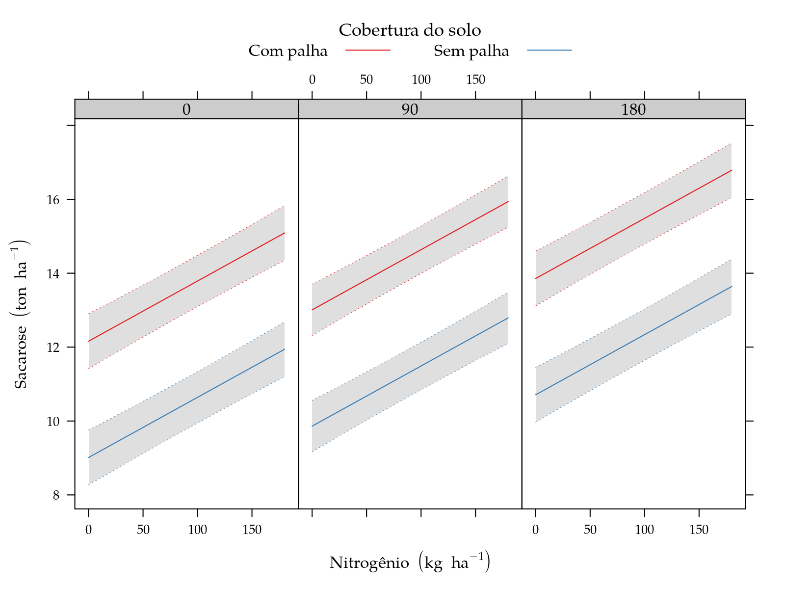
Teor de nitrogênio nas folhas
#-----------------------------------------------------------------------

leg$y <- "Teor de nitrogênio nas folhas"
sugarcane_straw$y <- sugarcane_straw$tfn

#-----------------------------------------------------------------------
# Scatter plots.

pk <- xyplot(y ~ K | palha, groups = N, data = sugarcane_straw,
             type = c("p", "a"),
             xlab = leg$K, ylab = leg$y,
             auto.key = list(title = leg$N,
                             cex.title = 1.1, columns = 5),
             strip = strip.custom(
                 strip.names = FALSE, strip.levels = TRUE,
                 factor.levels = c("Com palha", "Sem palha")))

pn <- xyplot(y ~ N | palha, groups = K, data = sugarcane_straw,
             type = c("p", "a"),
             xlab = leg$N, ylab = leg$y,
             auto.key = list(title = leg$K,
                             cex.title = 1.1, columns = 5),
             strip = strip.custom(
                 strip.names = FALSE, strip.levels = TRUE,
                 factor.levels = c("Com palha", "Sem palha")))

# grid.arrange(pn, pk)
# plot(pk)
plot(pn)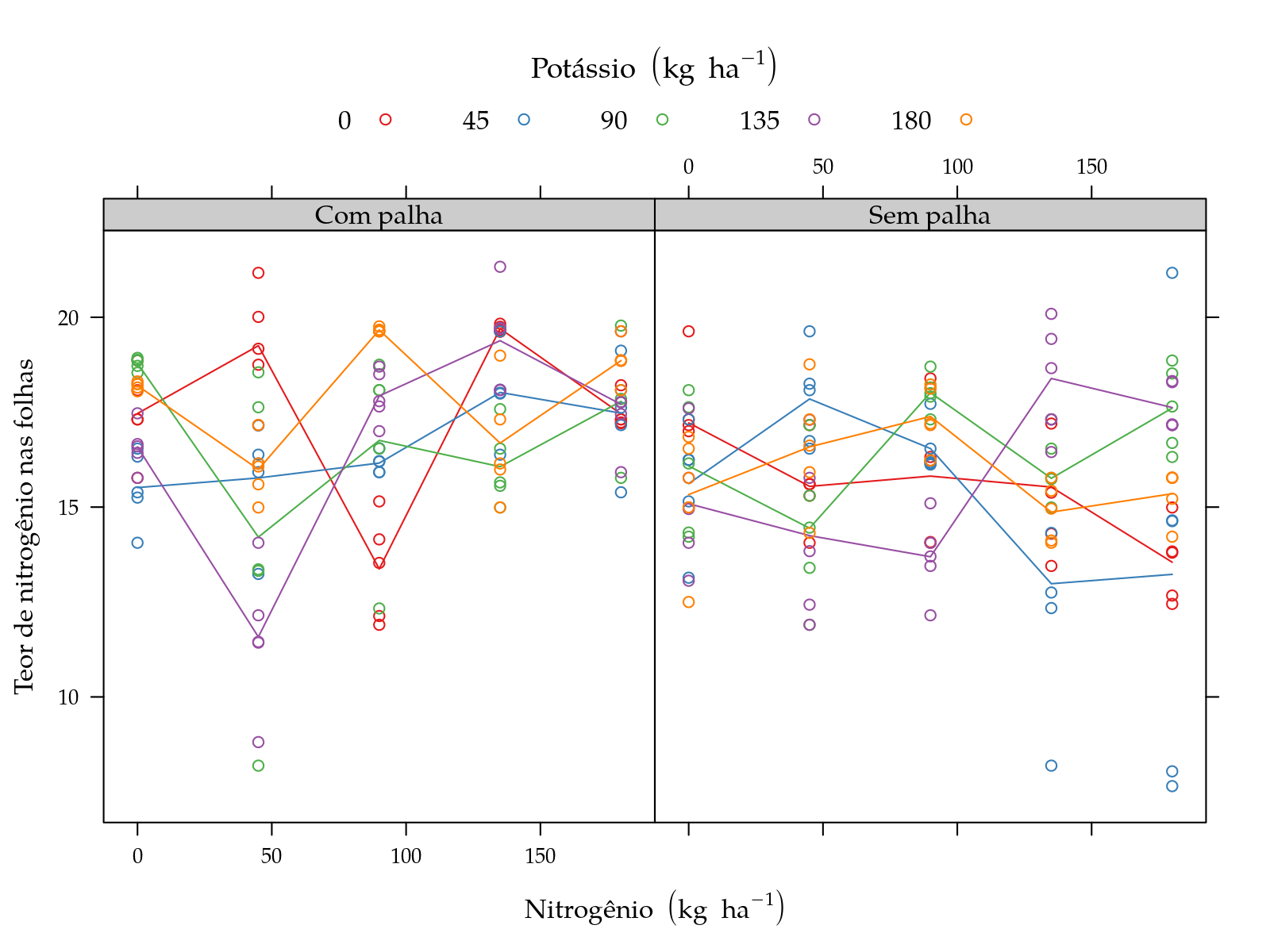
#-----------------------------------------------------------------------
# Model fitting.

# Saturated model.
m0 <- lmer(y ~ palha * nit * pot + (1 | bloc/ue),
           data = sugarcane_straw, REML = FALSE)

# Simple diagnostic.
plot(m0)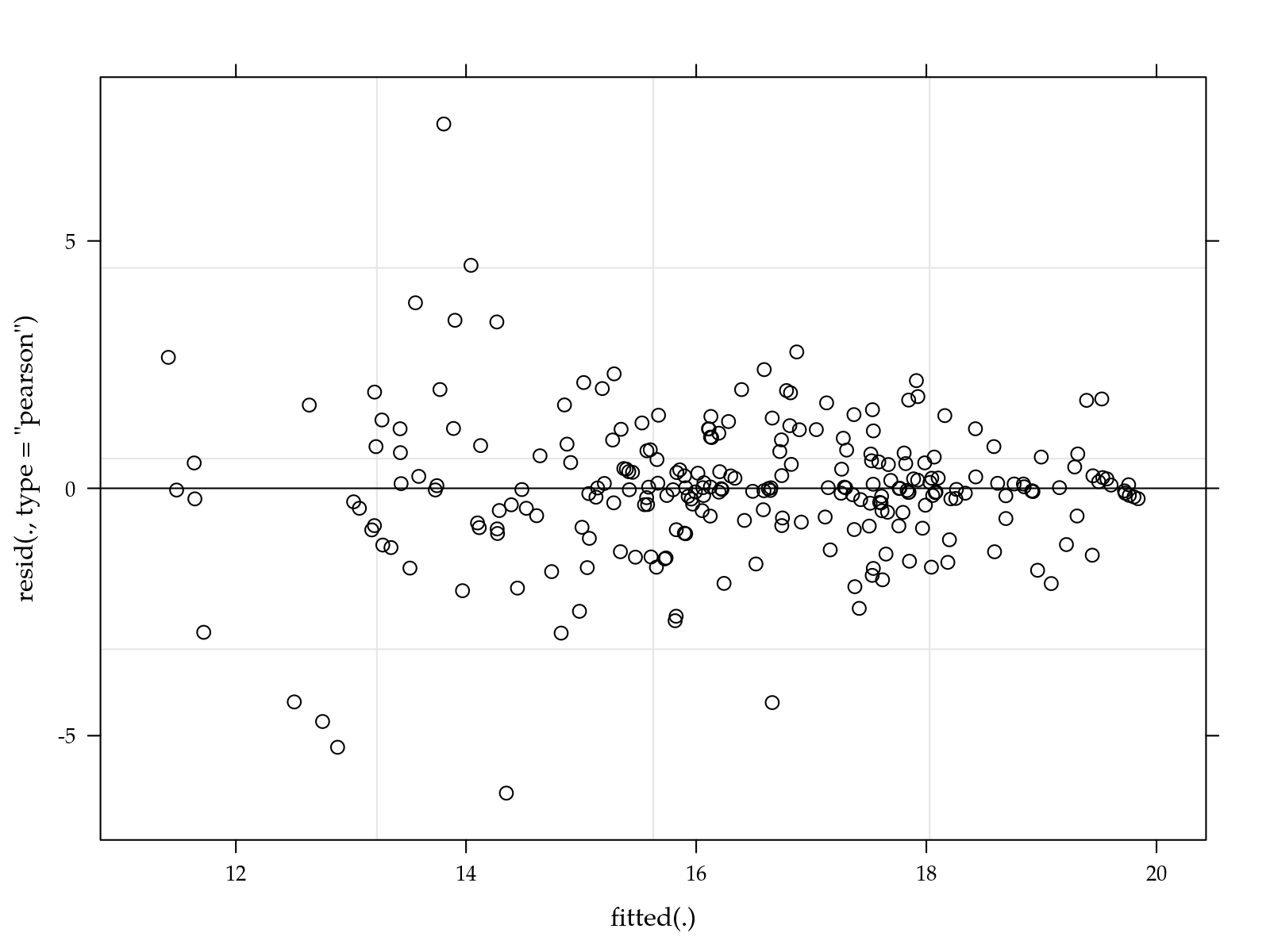
# qqnorm(residuals(m0, type = "pearson"))

# Estimates of the variance components.
VarCorr(m0)
## Groups Name Std.Dev.
## ue:bloc (Intercept) 0.31351
## bloc (Intercept) 0.17151
## Residual 1.43424# Tests for the fixed effects.
anova(m0)## Type III Analysis of Variance Table with Satterthwaite's method
## Sum Sq Mean Sq NumDF DenDF F value Pr(>F)
## palha 46.73 46.731 1 4.993 22.7179 0.0050493 **
## nit 48.12 12.031 4 239.995 5.8488 0.0001656 ***
## pot 26.94 6.734 4 239.995 3.2738 0.0122783 *
## palha:nit 75.22 18.804 4 239.995 9.1415 6.863e-07 ***
## palha:pot 24.78 6.194 4 239.995 3.0113 0.0188906 *
## nit:pot 370.94 23.184 16 239.995 11.2704 < 2.2e-16 ***
## palha:nit:pot 215.09 13.443 16 239.995 6.5353 3.461e-12 ***
## ---
## Signif. codes: 0 '***' 0.001 '**' 0.01 '*' 0.05 '.' 0.1 ' ' 1# Estimates of the effects and fitting measures.
# summary(m0)
# Final model.
mod <- m0
#-----------------------------------------------------------------------
# Fitted values.
# Experimental values to get estimates.
grid <- with(sugarcane_straw,
expand.grid(palha = levels(palha),
# N = seq(min(N), max(N), length.out = 10),
# K = seq(min(N), max(N), length.out = 3),
nit = levels(nit),
pot = levels(pot),
KEEP.OUT.ATTRS = FALSE))
# Matrix of fixed effects.
X <- model.matrix(terms(mod), data = cbind(grid, y = 0))
# Confidence intervals.
ci <- confint(glht(mod, linfct = X),
calpha = univariate_calpha())$confint
colnames(ci)[1] <- "fit"
grid <- cbind(grid, ci)
str(grid)## 'data.frame': 50 obs. of 6 variables:
## $ palha: Factor w/ 2 levels "1","2": 1 2 1 2 1 2 1 2 1 2 ...
## $ nit : Factor w/ 5 levels "0","45","90",..: 1 1 2 2 3 3 4 4 5 5 ...
## $ pot : Factor w/ 5 levels "0","45","90",..: 1 1 1 1 1 1 1 1 1 1 ...
## $ fit : num 17.5 17.2 19.3 15.5 13.4 ...
## $ lwr : num 16.2 15.9 18 14.3 12.1 ...
## $ upr : num 18.8 18.5 20.5 16.8 14.7 ...# Sample averages.
# averages <- aggregate(nobars(formula(mod)),
# data = sugarcane_straw, FUN = mean)
#
# xyplot(y ~ N | factor(K), groups = palha, data = averages,
# type = "o", as.table = TRUE)
xyplot(fit ~ pot | nit, groups = palha, data = grid,
as.table = TRUE, layout = c(NA, 1), type = "o",
xlab = leg$N, ylab = leg$y,
auto.key = list(title = leg$palha[1], cex.title = 1.1,
text = c(leg$palha[-1]), columns = 2,
points = FALSE, lines = TRUE),
uy = grid$upr, ly = grid$lwr,
desloc = 0.2 * scale(as.integer(grid$palha), scale = FALSE),
cty = "bars", length = 0.02,
alpha = 0.25, fill = "gray50",
prepanel = prepanel.cbH,
panel.groups = panel.cbH,
panel = panel.superpose)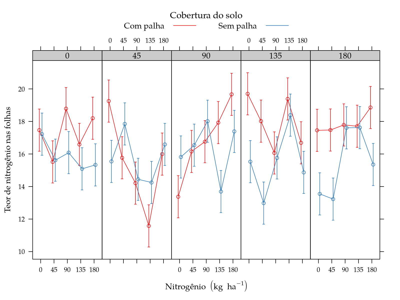
High order interactions present but no smooth effect of numeric factors.
Teor de potássio nas folhas
#-----------------------------------------------------------------------

leg$y <- "Teor de potássio nas folhas"
sugarcane_straw$y <- sugarcane_straw$tfk

#-----------------------------------------------------------------------
# Scatter plots.

pk <- xyplot(y ~ K | palha, groups = N, data = sugarcane_straw,
             type = c("p", "a"),
             xlab = leg$K, ylab = leg$y,
             auto.key = list(title = leg$N,
                             cex.title = 1.1, columns = 5),
             strip = strip.custom(
                 strip.names = FALSE, strip.levels = TRUE,
                 factor.levels = c("Com palha", "Sem palha")))

pn <- xyplot(y ~ N | palha, groups = K, data = sugarcane_straw,
             type = c("p", "a"),
             xlab = leg$N, ylab = leg$y,
             auto.key = list(title = leg$K,
                             cex.title = 1.1, columns = 5),
             strip = strip.custom(
                 strip.names = FALSE, strip.levels = TRUE,
                 factor.levels = c("Com palha", "Sem palha")))

# grid.arrange(pn, pk)
plot(pk)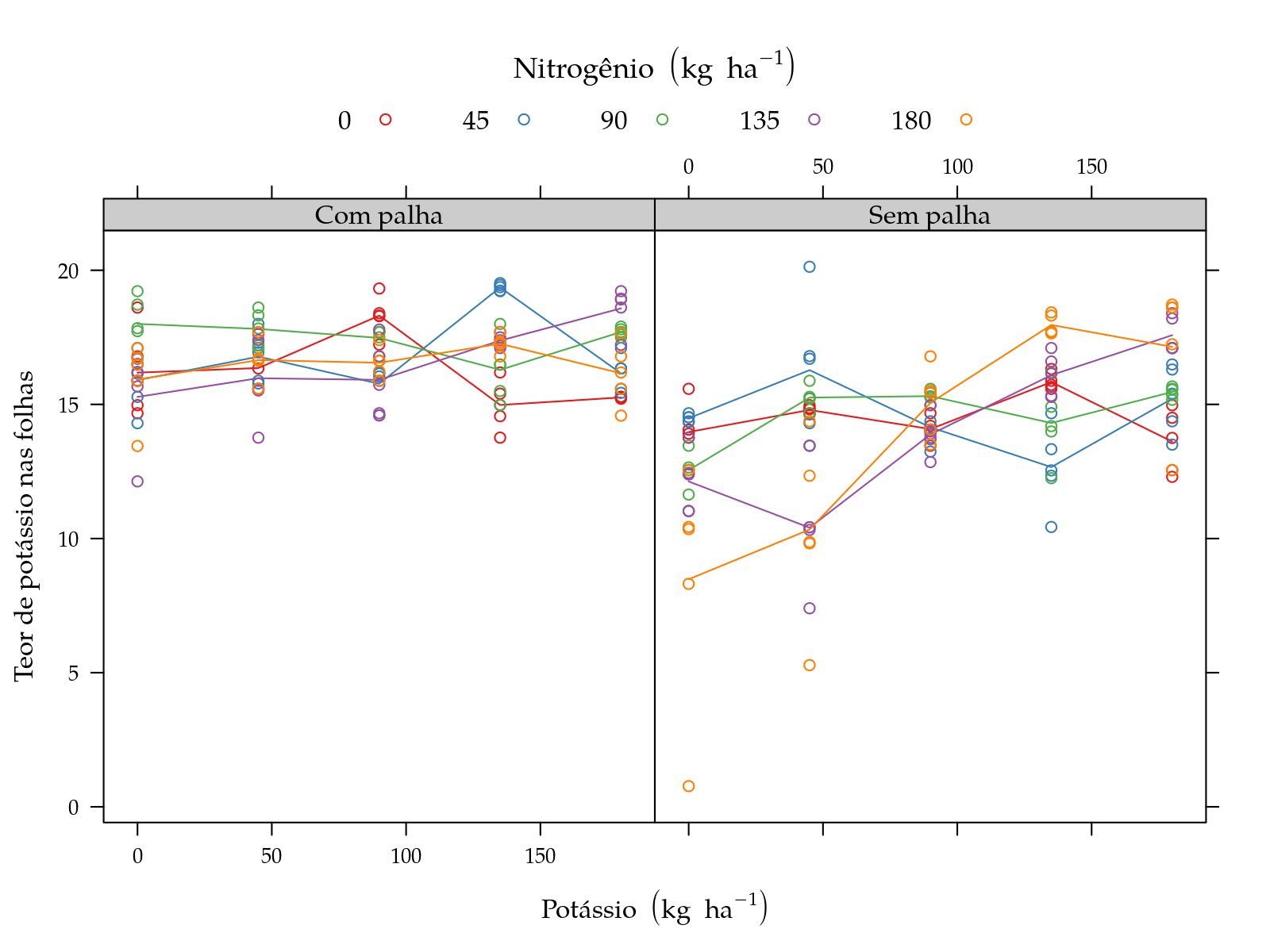
# plot(pn)#-----------------------------------------------------------------------
# Model fitting.
# Saturated model.
m0 <- lmer(y ~ palha * nit * pot + (1 | bloc/ue),
data = sugarcane_straw, REML = FALSE)
# Simple diagnostic.
plot(m0)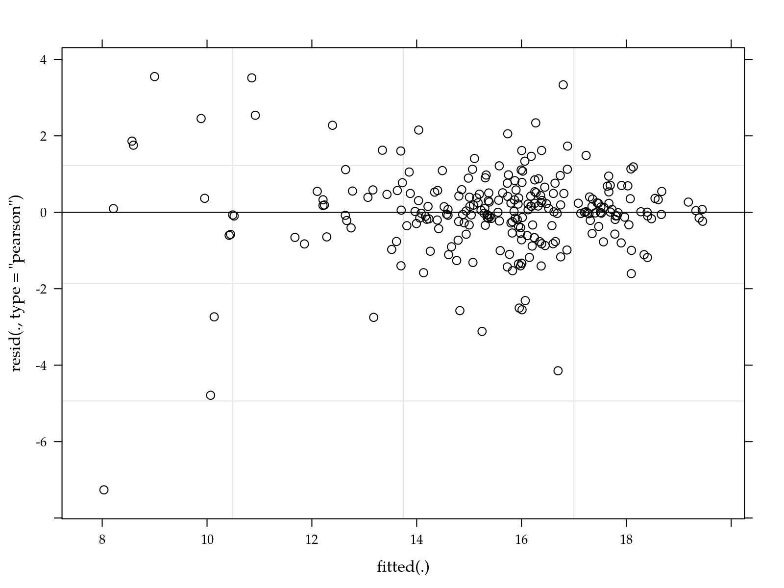
# qqnorm(residuals(m0, type = "pearson"))

# Estimates of the variance components.
VarCorr(m0)
## Groups Name Std.Dev.
## ue:bloc (Intercept) 0.26510
## bloc (Intercept) 0.15616
## Residual 1.15448# Tests for the fixed effects.
anova(m0)## Type III Analysis of Variance Table with Satterthwaite's method
## Sum Sq Mean Sq NumDF DenDF F value Pr(>F)
## palha 160.491 160.491 1 5 120.4145 0.0001093 ***
## nit 23.789 5.947 4 240 4.4621 0.0016998 **
## pot 139.954 34.988 4 240 26.2514 < 2.2e-16 ***
## palha:nit 9.992 2.498 4 240 1.8743 0.1156006
## palha:pot 71.767 17.942 4 240 13.4615 6.494e-10 ***
## nit:pot 281.636 17.602 16 240 13.2068 < 2.2e-16 ***
## palha:nit:pot 236.242 14.765 16 240 11.0781 < 2.2e-16 ***
## ---
## Signif. codes: 0 '***' 0.001 '**' 0.01 '*' 0.05 '.' 0.1 ' ' 1# Estimates of the effects and fitting measures.
# summary(m0)
# Final model.
mod <- m0
#-----------------------------------------------------------------------
# Fitted values.
# Experimental values to get estimates.
grid <- with(sugarcane_straw,
expand.grid(palha = levels(palha),
# N = seq(min(N), max(N), length.out = 10),
# K = seq(min(N), max(N), length.out = 3),
nit = levels(nit),
pot = levels(pot),
KEEP.OUT.ATTRS = FALSE))
# Matrix of fixed effects.
X <- model.matrix(terms(mod), data = cbind(grid, y = 0))
# Confidence intervals.
ci <- confint(glht(mod, linfct = X),
calpha = univariate_calpha())$confint
colnames(ci)[1] <- "fit"
grid <- cbind(grid, ci)
str(grid)## 'data.frame': 50 obs. of 6 variables:
## $ palha: Factor w/ 2 levels "1","2": 1 2 1 2 1 2 1 2 1 2 ...
## $ nit : Factor w/ 5 levels "0","45","90",..: 1 1 2 2 3 3 4 4 5 5 ...
## $ pot : Factor w/ 5 levels "0","45","90",..: 1 1 1 1 1 1 1 1 1 1 ...
## $ fit : num 16.2 14 15.9 14.5 18 ...
## $ lwr : num 15.1 12.9 14.9 13.4 17 ...
## $ upr : num 17.2 15 17 15.5 19 ...# Sample averages.
# averages <- aggregate(nobars(formula(mod)),
# data = sugarcane_straw, FUN = mean)
#
# xyplot(y ~ N | factor(K), groups = palha, data = averages,
# type = "o", as.table = TRUE)
xyplot(fit ~ pot | nit, groups = palha, data = grid,
as.table = TRUE, layout = c(NA, 1), type = "o",
xlab = leg$N, ylab = leg$y,
auto.key = list(title = leg$palha[1], cex.title = 1.1,
text = c(leg$palha[-1]), columns = 2,
points = FALSE, lines = TRUE),
uy = grid$upr, ly = grid$lwr,
desloc = 0.2 * scale(as.integer(grid$palha), scale = FALSE),
cty = "bars", length = 0.02,
alpha = 0.25, fill = "gray50",
prepanel = prepanel.cbH,
panel.groups = panel.cbH,
panel = panel.superpose)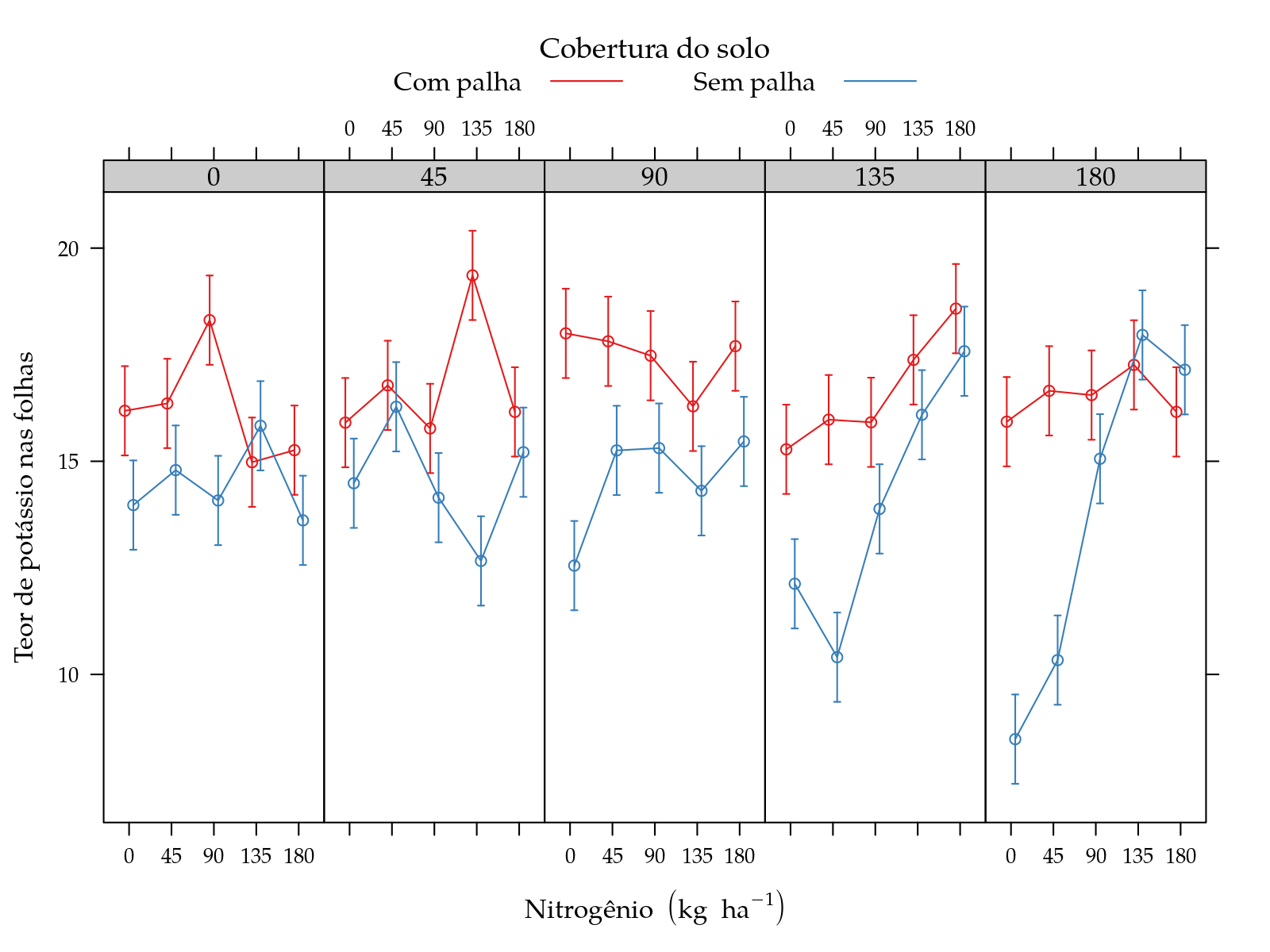
Session information
## quinta, 11 de julho de 2019, 20:05
## ----------------------------------------
## R version 3.6.1 (2019-07-05)
## Platform: x86_64-pc-linux-gnu (64-bit)
## Running under: Ubuntu 18.04.2 LTS
##
## Matrix products: default
## BLAS:   /usr/lib/x86_64-linux-gnu/blas/libblas.so.3.7.1
## LAPACK: /usr/lib/x86_64-linux-gnu/lapack/liblapack.so.3.7.1
##
## locale:
##  [1] LC_CTYPE=pt_BR.UTF-8       LC_NUMERIC=C
##  [3] LC_TIME=pt_BR.UTF-8        LC_COLLATE=en_US.UTF-8
##  [5] LC_MONETARY=pt_BR.UTF-8    LC_MESSAGES=en_US.UTF-8
##  [7] LC_PAPER=pt_BR.UTF-8       LC_NAME=C
##  [9] LC_ADDRESS=C               LC_TELEPHONE=C
## [11] LC_MEASUREMENT=pt_BR.UTF-8 LC_IDENTIFICATION=C
##
## attached base packages:
## [1] stats     graphics  grDevices utils     datasets  methods
## [7] base
##
## other attached packages:
##  [1] captioner_2.2.3     latticeExtra_0.6-28 RColorBrewer_1.1-2
##  [4] knitr_1.23          RDASC_0.0-6         multcomp_1.4-10
##  [7] TH.data_1.0-10      MASS_7.3-51.4       survival_2.44-1.1
## [10] mvtnorm_1.0-11      doBy_4.6-2          lmerTest_3.1-0
## [13] lme4_1.1-21         Matrix_1.2-17       gridExtra_2.3
## [16] lattice_0.20-38     wzRfun_0.81
##
## loaded via a namespace (and not attached):
##  [1] zoo_1.8-6           tidyselect_0.2.5    xfun_0.8
##  [4] purrr_0.3.2         splines_3.6.1       tcltk_3.6.1
##  [7] colorspace_1.4-1    htmltools_0.3.6     yaml_2.2.0
## [10] rpanel_1.1-4        rlang_0.4.0         pkgdown_1.3.0
## [13] pillar_1.4.2        nloptr_1.2.1        glue_1.3.1
## [16] plyr_1.8.4          stringr_1.4.0       munsell_0.5.0
## [19] commonmark_1.7      gtable_0.3.0        codetools_0.2-16
## [22] memoise_1.1.0       evaluate_0.14       Rcpp_1.0.1
## [25] scales_1.0.0        backports_1.1.4     desc_1.2.0
## [28] fs_1.3.1            ggplot2_3.2.0       digest_0.6.20
## [31] stringi_1.4.3       dplyr_0.8.3         numDeriv_2016.8-1.1
## [34] grid_3.6.1          rprojroot_1.3-2     tools_3.6.1
## [37] sandwich_2.5-1      magrittr_1.5        lazyeval_0.2.2
## [40] tibble_2.1.3        crayon_1.3.4        pkgconfig_2.0.2
## [43] xml2_1.2.0          assertthat_0.2.1    minqa_1.2.4
## [46] rmarkdown_1.13      roxygen2_6.1.1      R6_2.4.0
## [49] boot_1.3-23         nlme_3.1-140        compiler_3.6.1