Effect of fungicide sprays programs and pistachio hedging on sensitivity of Alternaria alternata to fluopyram, penthiopyrad and fluxapyroxad in Pistachio orchard of Tulare County, California
Paulo S. F. Lichtemberg, Ryan D. Puckett, Walmes M. Zeviani, Connor G. Cunningham & Themis J. Michailides
2019-07-11
ake_b-sensitivity.RmdSession Definition
# https://github.com/walmes/wzRfun
# devtools::install_github("walmes/wzRfun")

library(lattice)
library(latticeExtra)
library(plyr)
library(lme4)
library(lmerTest)
library(doBy)
library(multcomp)
library(wzRfun)library(RDASC)Exploratory Analysis
## 'data.frame':    10920 obs. of  11 variables:
##  $ yr  : int  2015 2015 2015 2015 2015 2015 2015 2015 2015 2015 ...
##  $ pop : Factor w/ 4 levels "A","B","C","D": 1 1 1 1 1 1 1 1 1 1 ...
##  $ hed : Factor w/ 2 levels "heavy","normal": 1 1 1 1 1 1 1 1 1 1 ...
##  $ tra : Factor w/ 4 levels "cnt","fon2","mer2",..: 2 2 2 2 2 2 2 2 2 2 ...
##  $ plot: Factor w/ 24 levels "1A","1AC","1B",..: 9 9 9 9 9 9 9 9 9 9 ...
##  $ iso : int  1 1 1 1 1 1 1 1 1 1 ...
##  $ fun : Factor w/ 3 levels "fd","fp","pe": 1 1 1 1 1 1 1 1 1 1 ...
##  $ dos : num  0 0 0.01 0.01 0.05 0.1 0.1 0.5 1 1 ...
##  $ rep : int  1 2 1 2 1 1 2 1 1 2 ...
##  $ d1  : int  1855 2263 2304 2317 2248 1854 2339 1791 1655 1521 ...
##  $ d2  : int  1871 2205 2317 2336 2193 1854 2436 1786 1686 1450 ...
# Short object names are handy.
sen <- ake_b$sensitivity
# Divide diameters by 100 to convert to milimeters. Calculate mean
# diameter (dm).
sen <- within(sen, {
# 500 is the plug size.
d1 <- (d1 - 500)/100
d2 <- (d2 - 500)/100
dm <- (d1 + d2)/2
ar <- pi * (dm/2)^2
})
# Population along years.
xtabs(~pop + yr, data = sen)## yr
## pop 2015 2016
## A 2478 0
## B 2478 0
## C 0 3318
## D 0 2646## fun fd fp pe
## yr hed tra
## 2015 heavy cnt 210 210 210
## fon2 210 210 210
## mer2 224 224 224
## mer3 182 182 182
## normal cnt 252 252 252
## fon2 182 182 182
## mer2 182 182 182
## mer3 210 210 210
## 2016 heavy cnt 476 476 476
## fon2 168 168 168
## mer2 182 182 182
## mer3 154 154 154
## normal cnt 448 448 448
## fon2 196 196 196
## mer2 210 210 210
## mer3 154 154 154# Number of isolates per factor combination.
with(sen,
ftable(tapply(iso,
INDEX = list(yr, hed, tra, fun),
FUN = function(x) {
length(unique(x))
})))## fd fp pe
##
## 2015 heavy cnt 15 15 15
## fon2 15 15 15
## mer2 16 16 16
## mer3 13 13 13
## normal cnt 18 18 18
## fon2 13 13 13
## mer2 13 13 13
## mer3 15 15 15
## 2016 heavy cnt 34 34 34
## fon2 12 12 12
## mer2 13 13 13
## mer3 11 11 11
## normal cnt 32 32 32
## fon2 14 14 14
## mer2 15 15 15
## mer3 11 11 11# Isolates x fungicide missing cells.
xt <- xtabs(complete.cases(cbind(dm, dos)) ~ iso + fun,
data = sen)
i <- xt == 0
sum(i)## [1] 15xt[rowSums(i) > 0, ]## fun
## iso fd fp pe
## 47 0 14 14
## 79 14 0 14
## 84 14 0 14
## 85 14 0 14
## 86 14 0 13
## 89 14 0 14
## 96 14 0 14
## 98 14 0 14
## 102 14 0 12
## 104 14 0 12
## 105 14 0 10
## 106 14 0 12
## 110 14 0 12
## 111 14 0 11
## 115 14 0 12xyplot(d2 ~ d1,
data = sen,
aspect = "iso",
xlab = "First diameter (mm)",
ylab = "Second diameter (mm)") +
layer(panel.abline(a = 0, b = 1))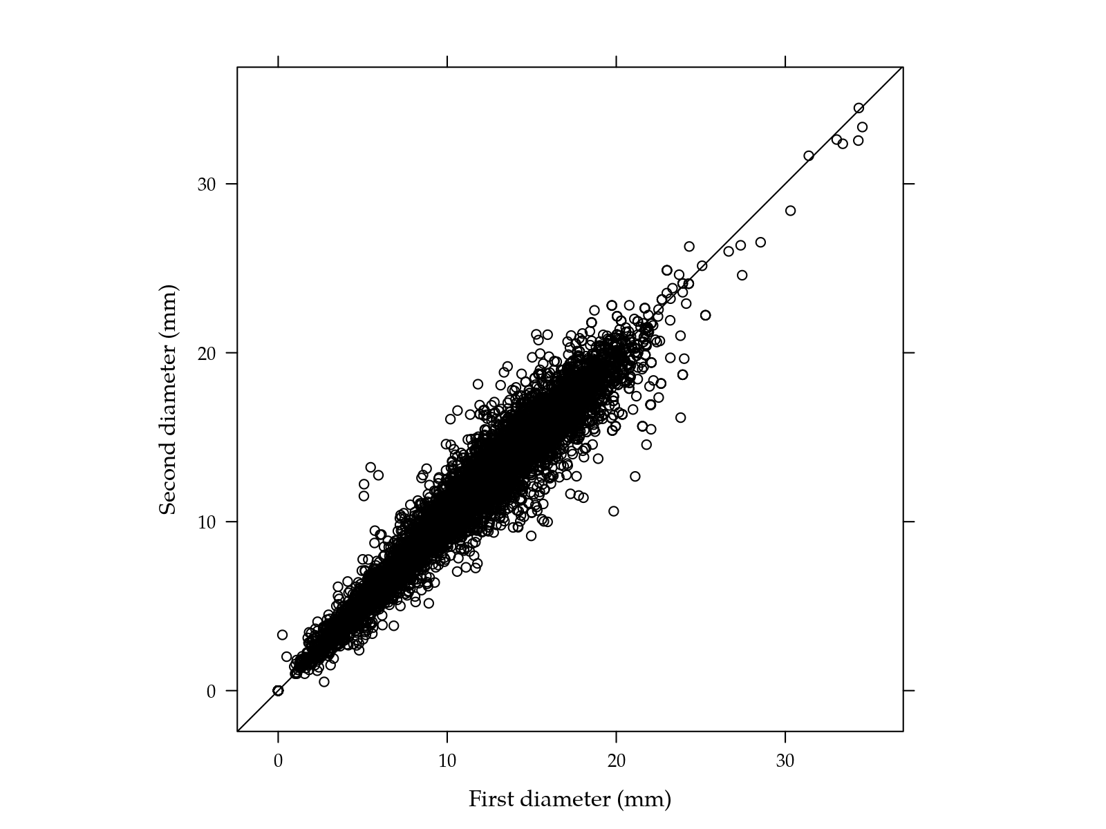
xyplot(d2 ~ d1 | iso,
       data = sen,
       aspect = "iso",
       groups = fun,
       strip = FALSE,
       as.table = TRUE,
       xlab = "First diameter (mm)",
       ylab = "Second diameter (mm)") +
    layer(panel.abline(a = 0, b = 1))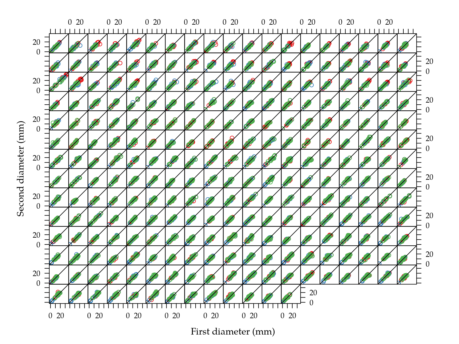
# Natural scales.
xyplot(dm ~ dos | iso,
       data = sen,
       groups = fun,
       type = c("p", "a"),
       strip = FALSE,
       as.table = TRUE,
       ylab = "Mean diameter (mm)",
       xlab = "Fungicide dose")

# Log-log scales.
xyplot(dm ~ dos | iso,
       scales = list(log = TRUE),
       data = sen,
       groups = fun,
       type = c("p", "a"),
       strip = FALSE,
       as.table = TRUE,
       ylab = "log Mean diameter (mm)",
       xlab = "log Fungicide dose")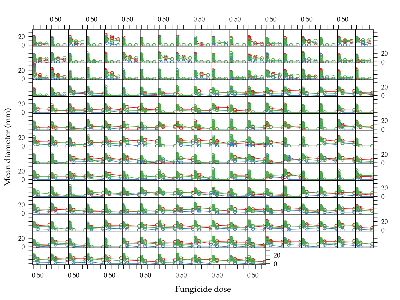
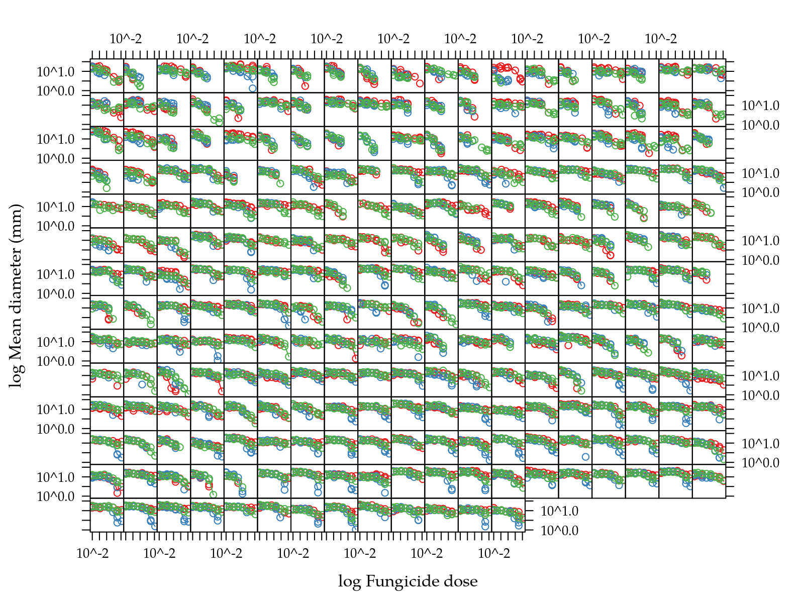
Figure 1: Scatter plots of mean diamenter as function of dose grouped by in vitro fungicide in natual scale (top) and log-log scale (bottom).
# 5th root of dose.
xyplot(dm ~ dos^0.2 | iso,
       data = sen,
       groups = fun,
       type = c("p", "a"),
       strip = FALSE,
       as.table = TRUE,
       ylab = "Mean diameter (mm)",
       xlab = "5th root fungicide dose")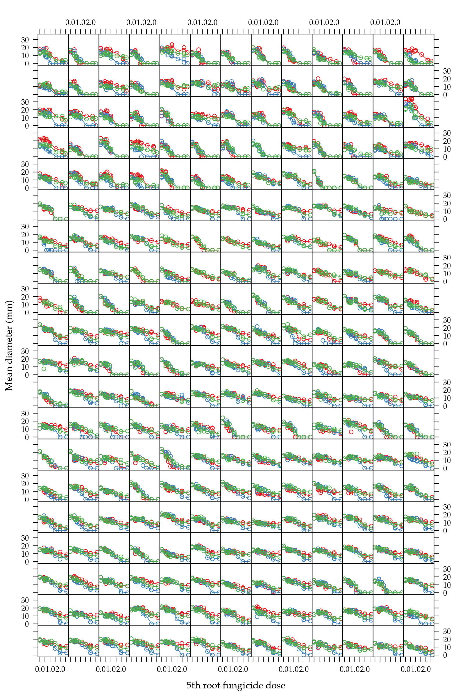
Figure 2: Scatter plot of mean diamenter as function of dose power 1/5 grouped by in vitro fungicide.
Figure 1 (top) shows that doses are very skewed. Figure 1 (bottom) shows that in the log-log scale there isn’t a linear relation between mean diameter and fungicide dose.
Figure 2 shows that, under the transformed 5th-root scale, doses levels are close to equally spaced. In fact, 0.2 was found by minimization of the variance of distance between doses (\(\sigma^2\)) a power transformation (\(p\)) of dose rescaled to a unit interval as described by the steps below \[ \begin{align*} z_i &= x_i^p\\ u_i &= \frac{z_i - \min(z)}{\max(z) -\min(z)}, \text{then } u_i \in [0, 1] \\ d_i &= u_{i+1} - u_{i}\\ \bar{d} &= \sum_{i=1}^{k-1} d_i/k \\ \sigma^2 &= \sum_{i=1}^{k-1} \frac{(d_i - \bar{d})^2}{k-2} \end{align*} \] where \(x\) are doses in natural scale, \(z\) are doses power transformed, \(u\) are scaled to a unit interval, \(d\) are diferences between doses, \(\bar{d}\) is the mean difference and \(\sigma^2\) is the variance of differences.
##  [1]   0.00   0.01   0.03   0.05   0.10   0.12   0.48   0.50   1.00
## [10]   1.92   7.68  10.00  30.72  50.00 100.00 122.88
# Variance of distance between doses scaled to a unit interval.
esp <- function(p) {
u <- x^p
u <- (u - min(u))
u <- u/max(u)
var(diff(u))
}
# Optimise de power parameter to the most equally spaced set.
op <- optimize(f = esp, interval = c(0, 1))
op$minimum## [1] 0.2091209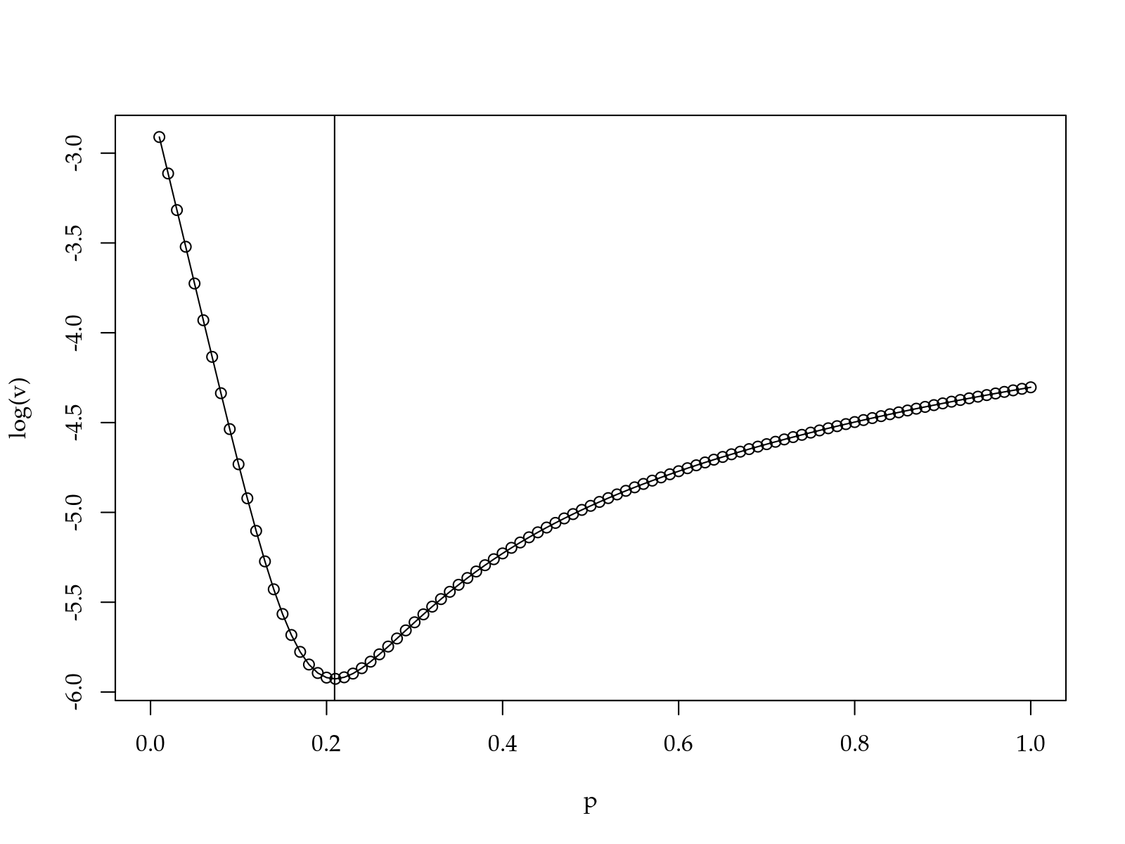
So \(x^{0.2}\) is the most equally spaced set obtained with a power transformation. Equally spaced levels are beneficial beacause reduce problems related to leverage.
Half Effective Concentration (EC50) Estimation
A cubic spline is function constructed of piecewise third-order polynomials which pass through a set of \(m + 1\) knots. These knots spans the observed domain of the continous factor \(x\), so the set of knots is \[ K = \{\xi_0, \xi_1, \ldots, \xi_m\}. \]
A function \(s(x)\) is a cubic spline if it is made of cubic polynomials \(s_{i}(x)\) in each interval \([x_{i-1}, x_{m}]\), \(i = 1, \ldots, m\).
Those adjacent cubic pylinomials pieces must bind and be smooth at the internal knots , so additional constrais are made to result in a composite continuous smooth function. Requering continous derivatives, we ensure that the resulting function is as smooth as possible.
For natural splines, two aditional boundary conditions are made \[ s^{''}_{1}(x) = 0, \quad s^{''}_{m}(x) = 0, \] that is, the pieces at borders aren’t cubic but instead linear.
Natural cubic splines were used to estimate the half effective concentration (EC50). A non linear model is usually applied in this context but wasn’t found a non linear model flexible enough to give a good fit either a satisfactory convergence rate. So, despite splines haven’t a model equation, they are vey flexible and numerical root-finding algorithms can e used to compute EG50 based on a linear interpolated function on a predicted grid. Also, area under the sensibility curve (AUSC) were computed by numerical integration under studied dose domain.
sen$iso <- factor(sen$iso, levels = sort(unique(sen$iso)))
sen$ue <- with(sen, interaction(iso, fun, drop = TRUE))
sen$doz <- sen$dos^0.2

# A data frame without dose.
senu <- unique(subset(sen,
                      select = c(ue, iso, fun, tra,
                                 hed, pop, yr, plot)))

# Splines.
library(splines)

# Function for fitting splines.
fitting <- function(x) {
    x <- na.omit(x)
    if (nrow(x) > 4) {
        n0 <- lm(dm ~ ns(doz, df = 3), data = x)
        yfit <- predict(n0, newdata = pred)
        # n0 <- glm(dm + 0.01 ~ ns(doz, df = 3), data = x,
        #           family = gaussian(link = log))
        # yfit <- predict(n0, newdata = pred, type = "response")
        # yr <- range(x$dm)
        return(cbind(xfit = pred$doz, yfit = yfit))
    } else {
        NULL
    }
}

# Values of dose to predict diameter.
pred <- data.frame(doz = seq(0, max(sen$doz), length.out = 30))

# Appling to all experimental unit.
res <- ddply(sen, .(ue), .fun = fitting)

# Merge to pair `iso` and `fun`.
res <- merge(res, senu, by = "ue")
# Estimatinf EC50 and area under curve.
get_ec50 <- function(x, y, interval = c(0, max(sen$doz))) {
fa <- approxfun(x = x, y = y)
int <- integrate(fa,
lower = 0,
upper = max(sen$doz))$value
mxm <- optimize(fa, interval = interval, maximum = TRUE)
ymid <- mxm[[2]]/2
u <- try(uniroot(f = function(x) fa(x) - ymid,
interval = interval),
silent = TRUE)
if (class(u) == "try-error") {
return(c(ec50 = NA, ev50 = NA, auc = int))
}
else {
return(c(ec50 = u$root, ev50 = ymid, auc = int))
}
}
# EC50 and AUC for each experimental unit.
ec <- ddply(res, .(ue), .fun = function(x) get_ec50(x$xfit, x$yfit))
str(ec)## 'data.frame': 765 obs. of 4 variables:
## $ ue : Factor w/ 780 levels "1.fd","2.fd",..: 1 2 3 4 5 6 7 8 9 10 ...
## $ ec50: num 1.19 0.568 2.006 0.717 NA ...
## $ ev50: num 8.75 7.79 8.07 7.73 NA ...
## $ auc : num 23.24 6.55 31.68 8.02 47.74 ...# Proportion of not estimated EC50 and AUC.
cbind(AUC = sum(is.na(ec$auc)),
EC50 = sum(is.na(ec$ev50)))/nrow(ec)## AUC EC50
## [1,] 0 0.124183
xyplot(auc ~ ec50,
       data = ec,
       type = c("p", "smooth"),
       ylab = "Area under the fitted curve",
       xlab = expression("Estimated" ~ EC[50]))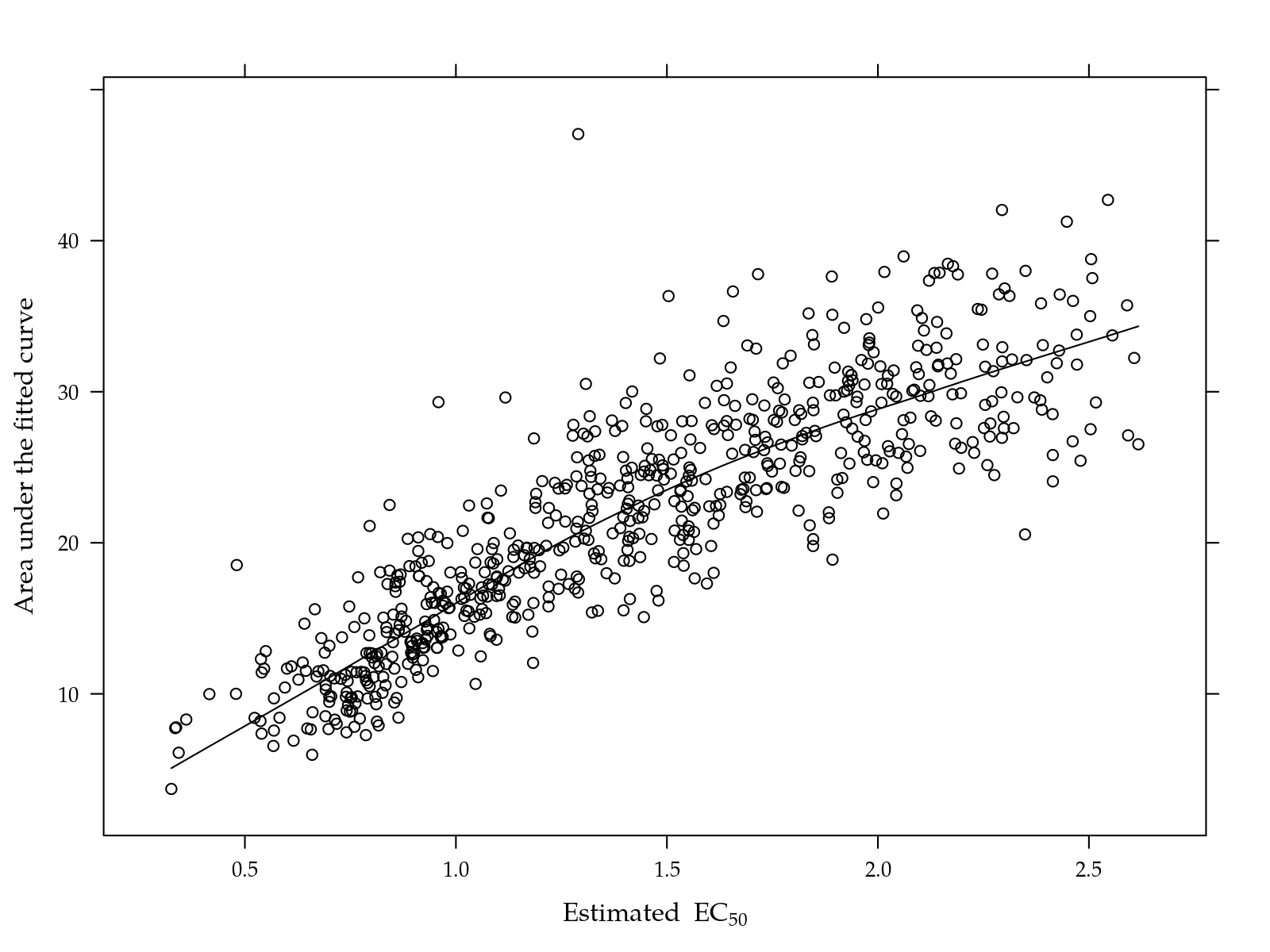
Figure 3: Area under the fitted curve as a function of the EC50 for those isolates where EC50 were estimated.
# Correlation among variables.
cor(ec[, -1], use = "complete")
## ec50 ev50 auc
## ec50 1.000000000 -0.000288753 0.8660755
## ev50 -0.000288753 1.000000000 0.4132968
## auc 0.866075500 0.413296809 1.0000000## 'data.frame': 780 obs. of 11 variables:
## $ ue : Factor w/ 780 levels "1.fd","2.fd",..: 1 2 3 4 5 6 7 8 9 10 ...
## $ ec50: num 1.19 0.568 2.006 0.717 NA ...
## $ ev50: num 8.75 7.79 8.07 7.73 NA ...
## $ auc : num 23.24 6.55 31.68 8.02 47.74 ...
## $ iso : Factor w/ 260 levels "1","2","3","4",..: 1 2 3 4 5 6 7 8 9 10 ...
## $ fun : Factor w/ 3 levels "fd","fp","pe": 1 1 1 1 1 1 1 1 1 1 ...
## $ tra : Factor w/ 4 levels "cnt","fon2","mer2",..: 2 2 2 2 1 2 2 1 3 3 ...
## $ hed : Factor w/ 2 levels "heavy","normal": 1 1 1 1 1 1 1 1 1 1 ...
## $ pop : Factor w/ 4 levels "A","B","C","D": 1 1 1 1 1 1 1 1 1 1 ...
## $ yr : int 2015 2015 2015 2015 2015 2015 2015 2015 2015 2015 ...
## $ plot: Factor w/ 24 levels "1A","1AC","1B",..: 9 9 9 9 10 21 21 22 5 5 ...# View the results.
L <- split(ec, ec$iso)
xyplot(dm ~ dos^0.2 | iso,
data = sen,
groups = fun,
cex = 0.4,
strip = FALSE,
as.table = TRUE,
auto.key = list(columns = 3,
title = "In vitro fungicide",
cex.title = 1.1),
xlab = "In vitro fungicide dose 5th root",
ylab = "Mean diameter (mm)") +
as.layer(xyplot(yfit ~ xfit | iso,
groups = fun,
data = res,
type = "l")) +
layer({
with(L[[which.packet()]], {
cl <- trellis.par.get()$superpose.symbol$col[as.integer(fun)]
panel.segments(x0 = ec50,
y0 = ev50,
x1 = ec50,
y1 = 0,
col = "gray50")
panel.segments(x0 = ec50,
y0 = ev50,
x1 = 0,
y1 = ev50,
col = "gray50")
panel.points(x = ec50,
y = ev50,
pch = 19,
cex = 0.6,
col = cl)
})
})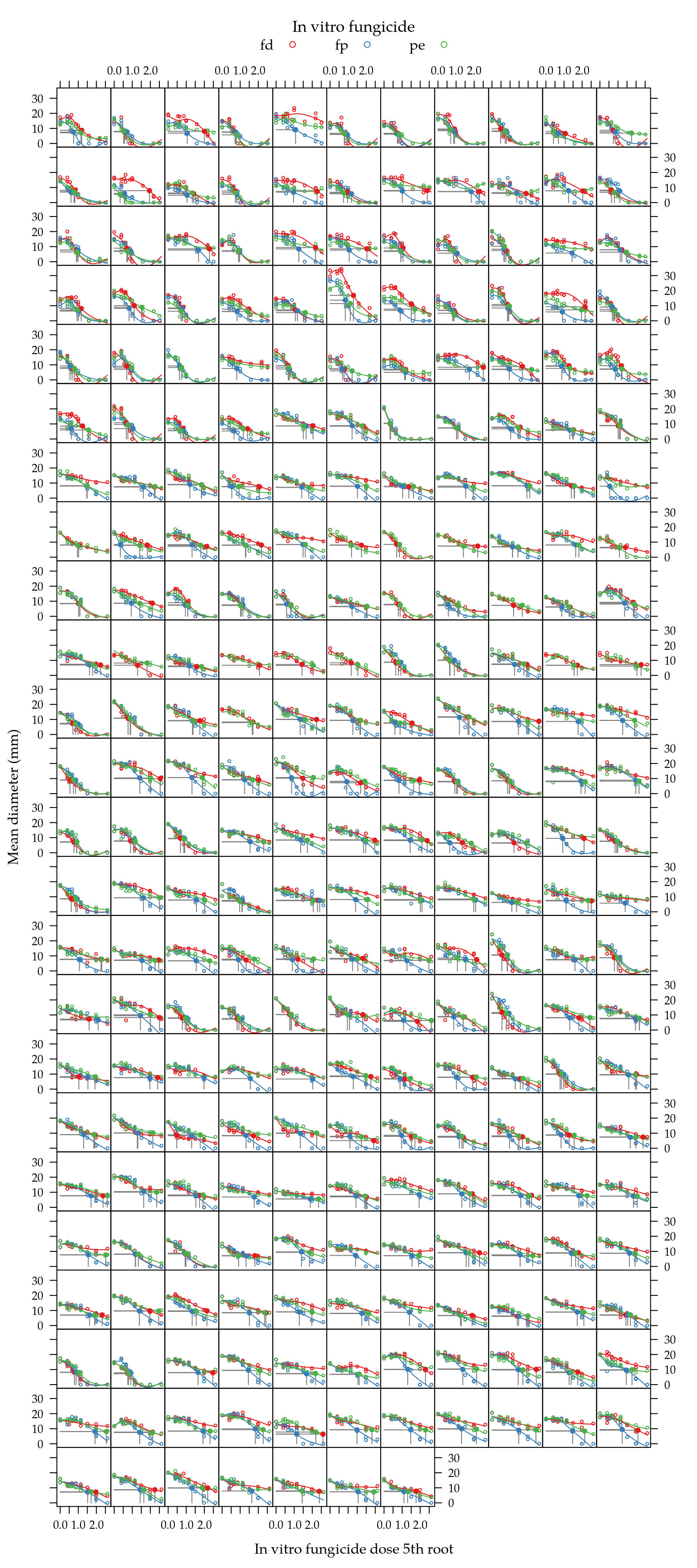
Figure 4: Mean diameter as function of fungicide dose 5th root for each isolate. Solid line is the natural cubic spline fitted for each fungicide in each isolate. Gray straight line indicates the EC50 on each curve.
# Subseting.
set.seed(123)
i <- sample(levels(sen$iso), size = 40)
i <- as.character(sort(as.integer(i)))
L <- L[i]

xyplot(dm ~ dos^0.2 | iso,
       data = sen,
       subset = iso %in% i,
       groups = fun,
       cex = 0.4,
       strip = FALSE,
       as.table = TRUE,
       auto.key = list(columns = 3,
                       title = "In vitro fungicide",
                       cex.title = 1.1),
       xlab = "In vitro fungicide dose 5th root",
       ylab = "Mean diameter (mm)") +
    as.layer(xyplot(yfit ~ xfit | iso,
                    groups = fun,
                    data = res,
                    subset = iso %in% i,
                    type = "l")) +
    layer({
        with(L[[which.packet()]], {
            cl <- trellis.par.get()$superpose.symbol$col[as.integer(fun)]
            panel.segments(x0 = ec50,
                           y0 = ev50,
                           x1 = ec50,
                           y1 = 0,
                           col = "gray50")
            panel.segments(x0 = ec50,
                           y0 = ev50,
                           x1 = 0,
                           y1 = ev50,
                           col = "gray50")
            panel.points(x = ec50,
                         y = ev50,
                         pch = 19,
                         cex = 0.6,
                         col = cl)
        })
    })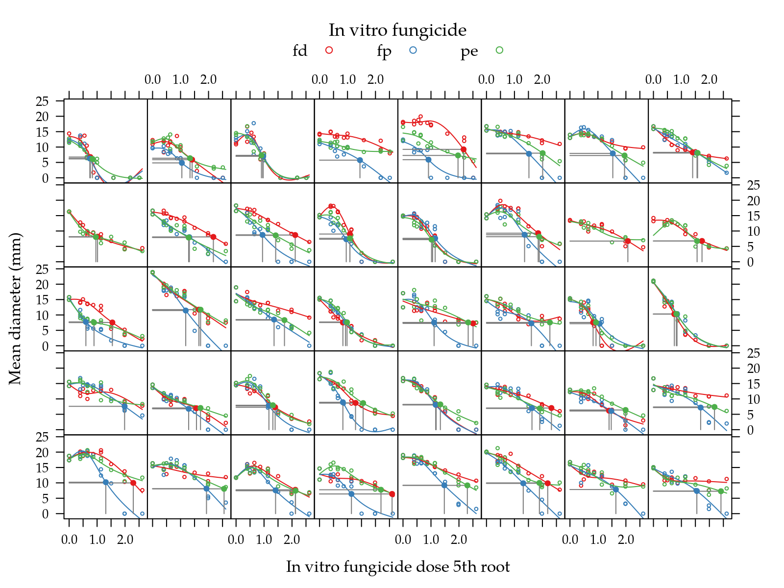
Figure 5: Mean diameter as function of fungicide dose 5th root for a random sample of isolates. Solid line is the natural cubic spline fitted for each fungicide in each isolate. Gray straight line indicates the EC50 on each curve.
Analysis of Area Under Sensitivity Curve
p <- xyplot(ec50 ~ fun | pop + hed,
            groups = tra,
            data = ec[!is.na(ec$ec50), ],
            type = c("p", "a"))
useOuterStrips(p)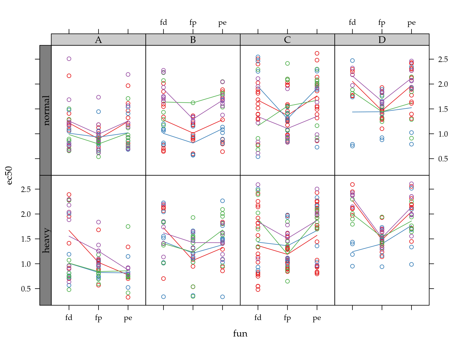
p <- xyplot(auc ~ fun | pop + hed,
            groups = tra,
            data = ec[!is.na(ec$auc), ],
            type = c("p", "a"))
useOuterStrips(p)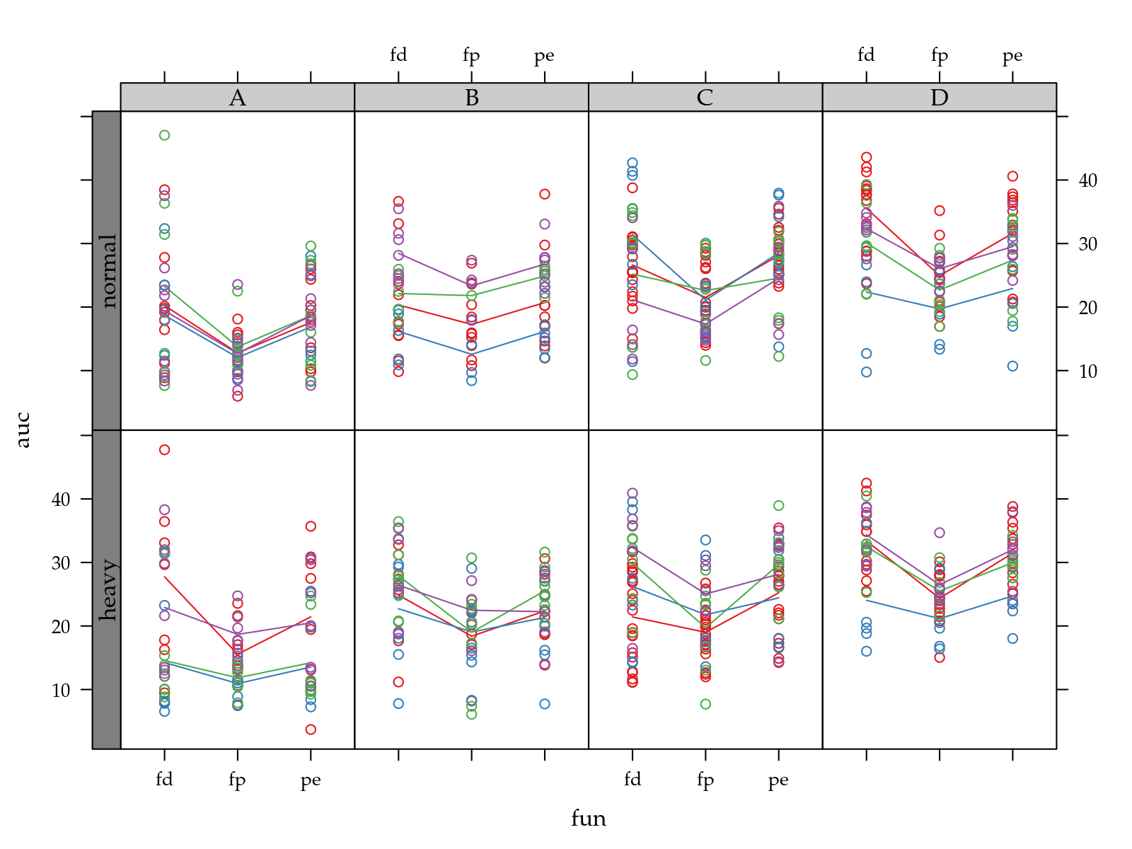
p <- xyplot(auc ~ tra | pop + hed,
            groups = fun,
            data = ec[!is.na(ec$auc), ],
            type = c("p", "a"))
useOuterStrips(p)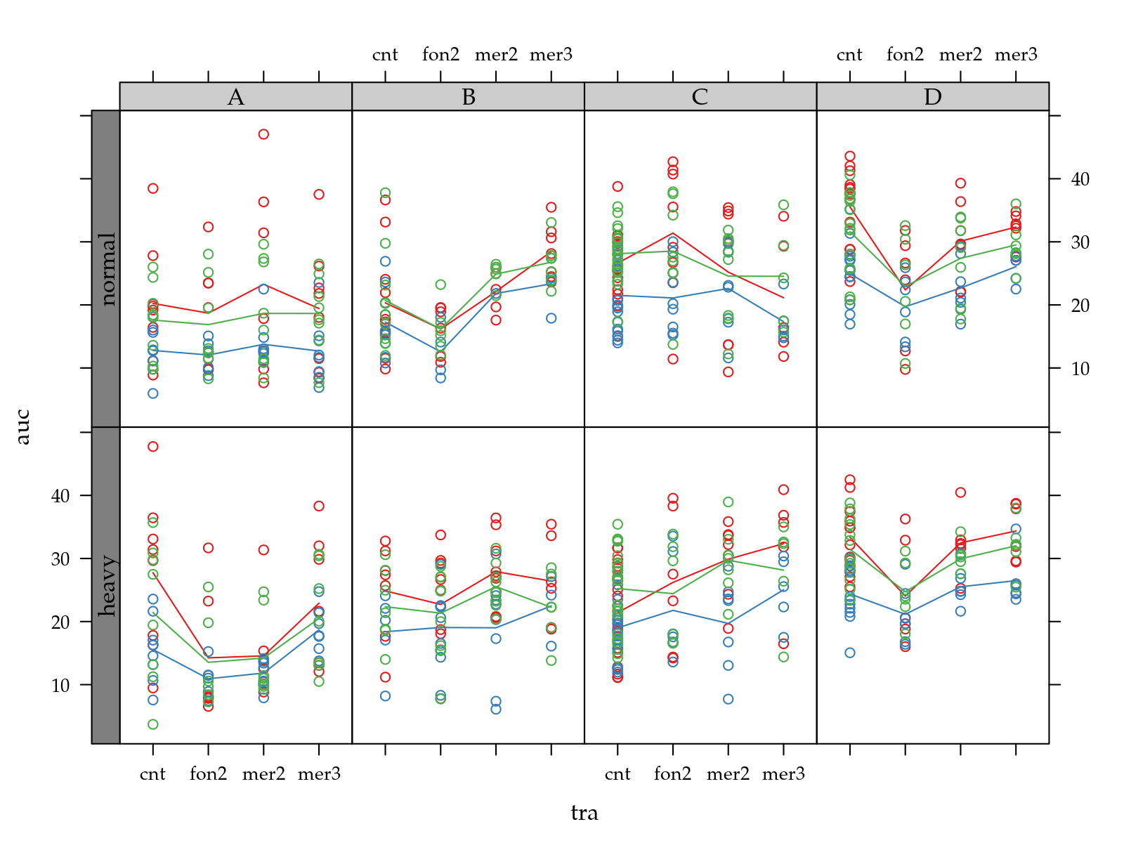
p <- xyplot(auc ~ pop | tra + fun,
            groups = hed,
            data = ec[!is.na(ec$auc), ],
            type = c("p", "a"))
useOuterStrips(p)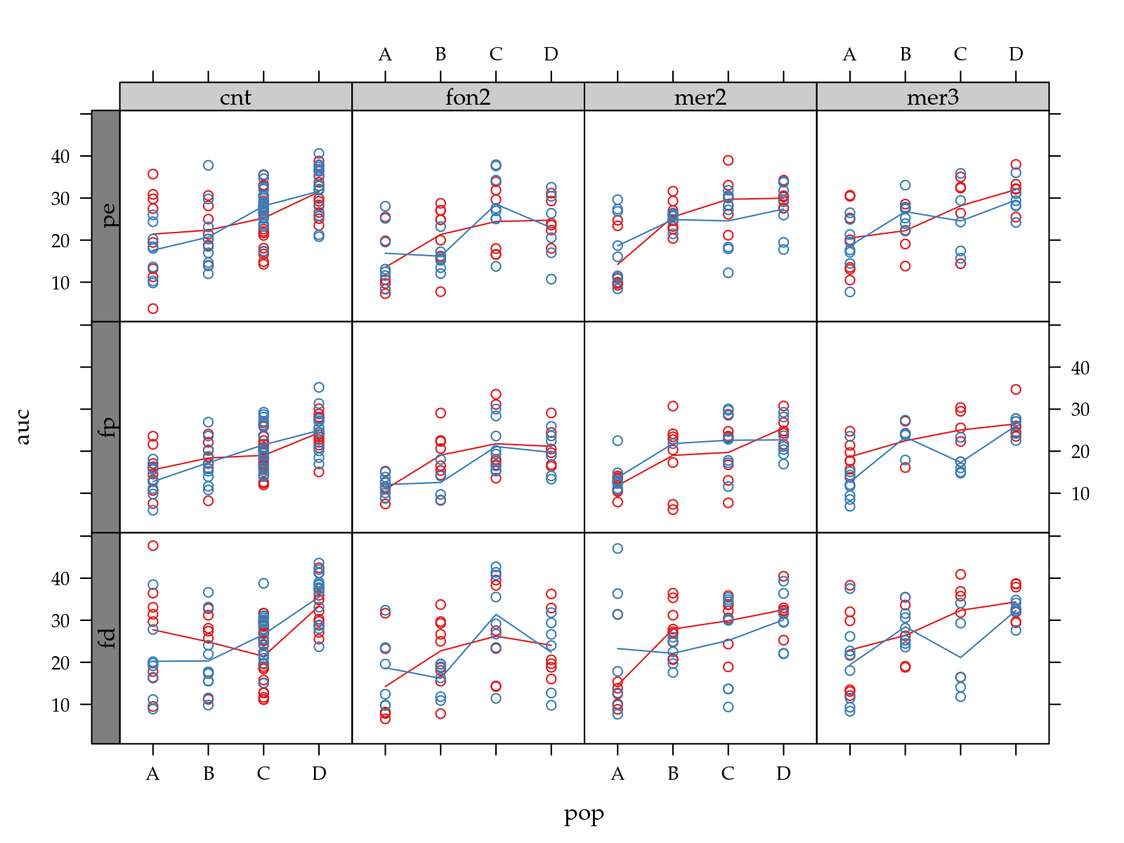
#-----------------------------------------------------------------------
# Creates block and treatment cell factors.

ec$blk <- factor(as.integer(as.integer(substr(ec$plot, 0, 1)) > 2))
ec$cell <- with(ec, interaction(yr, blk, hed, tra, drop = TRUE))

# Number of isolates per cell combination.
ftable(xtabs(~pop + hed + tra, data = ec))/3
## tra cnt fon2 mer2 mer3
## pop hed
## A heavy 8 6 7 7
## normal 8 7 8 8
## B heavy 7 9 9 6
## normal 10 6 5 7
## C heavy 22 6 7 5
## normal 18 8 8 5
## D heavy 12 6 6 6
## normal 14 6 7 6# ddply(ec,
# ~yr + pop + tra + hed,
# function(x) {
# nlevels(droplevels(x$iso))
# })
ec <- arrange(df = ec, yr, blk, hed, tra, iso, fun)
str(ec)## 'data.frame': 780 obs. of 13 variables:
## $ ue : Factor w/ 780 levels "1.fd","2.fd",..: 5 265 525 13 273 533 14 274 534 24 ...
## $ ec50: num NA 1.078 NA 1.951 0.569 ...
## $ ev50: num NA 9.14 NA 7.91 6.05 ...
## $ auc : num 47.74 21.63 35.69 29.67 7.57 ...
## $ iso : Factor w/ 260 levels "1","2","3","4",..: 5 5 5 13 13 13 14 14 14 24 ...
## $ fun : Factor w/ 3 levels "fd","fp","pe": 1 2 3 1 2 3 1 2 3 1 ...
## $ tra : Factor w/ 4 levels "cnt","fon2","mer2",..: 1 1 1 1 1 1 1 1 1 1 ...
## $ hed : Factor w/ 2 levels "heavy","normal": 1 1 1 1 1 1 1 1 1 1 ...
## $ pop : Factor w/ 4 levels "A","B","C","D": 1 1 1 1 1 1 1 1 1 1 ...
## $ yr : int 2015 2015 2015 2015 2015 2015 2015 2015 2015 2015 ...
## $ plot: Factor w/ 24 levels "1A","1AC","1B",..: 10 10 10 6 6 6 6 6 6 2 ...
## $ blk : Factor w/ 2 levels "0","1": 1 1 1 1 1 1 1 1 1 1 ...
## $ cell: Factor w/ 32 levels "2015.0.heavy.cnt",..: 1 1 1 1 1 1 1 1 1 1 ...2015
#-----------------------------------------------------------------------

ec15 <- subset(ec, yr == 2015)

# Mixed effects model.
m0 <- lmer(auc ~ blk + (1 | iso) + (pop + tra + hed + fun)^2,
           data = ec15,
           REML = FALSE)

# r <- residuals(m0)
# f <- fitted(m0)
# useOuterStrips(qqmath(~r | pop + tra, data = ec15))
# useOuterStrips(xyplot(r ~ f| pop + tra, data = ec15))

# Wald tests for the fixed effects.
anova(m0)
## Type III Analysis of Variance Table with Satterthwaite's method
## Sum Sq Mean Sq NumDF DenDF F value Pr(>F)
## blk 22.96 22.96 1 118.52 1.2562 0.26464
## pop 335.83 335.83 1 120.44 18.3731 3.68e-05 ***
## tra 198.95 66.32 3 119.62 3.6281 0.01503 *
## hed 18.71 18.71 1 119.88 1.0237 0.31367
## fun 1888.83 944.42 2 223.60 51.6684 < 2.2e-16 ***
## pop:tra 78.44 26.15 3 119.75 1.4304 0.23732
## pop:hed 11.14 11.14 1 119.79 0.6095 0.43653
## pop:fun 32.82 16.41 2 223.58 0.8978 0.40894
## tra:hed 46.05 15.35 3 119.30 0.8398 0.47467
## tra:fun 86.53 14.42 6 223.16 0.7890 0.57938
## hed:fun 39.52 19.76 2 223.19 1.0811 0.34100
## ---
## Signif. codes: 0 '***' 0.001 '**' 0.01 '*' 0.05 '.' 0.1 ' ' 1# A simpler model.
m1 <- update(m0, auc ~ blk + (1 | iso) + (pop + tra + fun))
# LRT between nested models.
anova(m1, m0)## Data: ec15
## Models:
## m1: auc ~ blk + (1 | iso) + pop + tra + fun
## m0: auc ~ blk + (1 | iso) + (pop + tra + hed + fun)^2
## Df AIC BIC logLik deviance Chisq Chi Df Pr(>Chisq)
## m1 10 2185.8 2224.1 -1082.9 2165.8
## m0 28 2204.7 2311.8 -1074.4 2148.7 17.128 18 0.5143# Parameter estimates.
summary(m1)## Linear mixed model fit by maximum likelihood . t-tests use
## Satterthwaite's method [lmerModLmerTest]
## Formula: auc ~ blk + (1 | iso) + pop + tra + fun
## Data: ec15
##
## AIC BIC logLik deviance df.resid
## 2185.8 2224.1 -1082.9 2165.8 329
##
## Scaled residuals:
## Min 1Q Median 3Q Max
## -2.6358 -0.5810 -0.0094 0.5269 3.1901
##
## Random effects:
## Groups Name Variance Std.Dev.
## iso (Intercept) 31.63 5.624
## Residual 18.94 4.352
## Number of obs: 339, groups: iso, 118
##
## Fixed effects:
## Estimate Std. Error df t value Pr(>|t|)
## (Intercept) 20.52206 1.33643 133.72455 15.356 < 2e-16 ***
## blk1 -1.06013 1.15418 119.08963 -0.919 0.360209
## popB 4.52162 1.15169 119.51086 3.926 0.000145 ***
## trafon2 -3.11213 1.58679 117.54578 -1.961 0.052212 .
## tramer2 0.02077 1.58044 118.92826 0.013 0.989537
## tramer3 1.82956 1.59329 119.03816 1.148 0.253152
## funfp -6.09716 0.59459 224.52712 -10.254 < 2e-16 ***
## funpe -1.81643 0.56822 222.15000 -3.197 0.001592 **
## ---
## Signif. codes: 0 '***' 0.001 '**' 0.01 '*' 0.05 '.' 0.1 ' ' 1
##
## Correlation of Fixed Effects:
## (Intr) blk1 popB trafn2 tramr2 tramr3 funfp
## blk1 -0.309
## popB -0.402 -0.125
## trafon2 -0.529 -0.029 -0.010
## tramer2 -0.536 -0.073 0.036 0.461
## tramer3 -0.553 -0.031 0.046 0.456 0.461
## funfp -0.224 -0.013 0.034 0.004 0.012 0.018
## funpe -0.213 -0.002 0.002 0.000 -0.003 0.000 0.481# Least squares means.
i <- c("pop", "tra", "fun")
L <- lapply(i,
FUN = function(term){
L <- LSmeans(m1, effect = term)
rownames(L$L) <- L$grid[, 1]
a <- apmc(L$L, m1, focus = term)
names(a)[1] <- "level"
a <- cbind(term = term, a)
return(a)
})
res <- ldply(L)
# str(res)
i <- c("Population",
expression("Fungicide" ~ italic("in vivo")),
expression("Fungicide" ~ italic("in vitro")))resizePanels(
segplot(level ~ lwr + upr | term,
centers = fit,
data = res,
as.table = TRUE,
draw = FALSE,
layout = c(1, NA),
scales = list(y = list(relation = "free")),
xlab = "Area under isolate sensitivity curve",
ylab = "Levels of each factor",
strip = strip.custom(factor.levels = i),
cld = res$cld) +
layer(panel.text(x = centers,
y = z,
labels = sprintf("%0.1f %s", centers, cld),
pos = 3)),
h = sapply(L, nrow)
)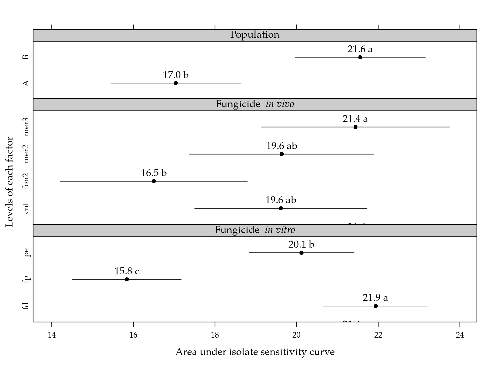
Figure 6: Area under isolate sensitivity curve for levels of population, in vivo fungicide and in vitro fungicide. Pairs of means in a factor followed by the same letter are not statistically different at 5% significance level.
2016
#-----------------------------------------------------------------------

ec16 <- subset(ec, yr == 2016)

# Mixed effects model.
m0 <- lmer(auc ~ blk + (1 | iso) + (pop + tra + hed + fun)^2,
           data = ec16,
           REML = FALSE)

# r <- residuals(m0)
# f <- fitted(m0)
# useOuterStrips(qqmath(~r | pop + tra, data = ec15))
# useOuterStrips(xyplot(r ~ f| pop + tra, data = ec15))

# Wald tests for the fixed effects.
anova(m0)
## Type III Analysis of Variance Table with Satterthwaite's method
## Sum Sq Mean Sq NumDF DenDF F value Pr(>F)
## blk 0.80 0.80 1 142 0.0739 0.7861916
## pop 87.89 87.89 1 142 8.1096 0.0050571 **
## tra 62.56 20.85 3 142 1.9239 0.1284132
## hed 8.89 8.89 1 142 0.8200 0.3667068
## fun 2640.46 1320.23 2 284 121.8116 < 2.2e-16 ***
## pop:tra 164.04 54.68 3 142 5.0451 0.0023725 **
## pop:hed 3.79 3.79 1 142 0.3496 0.5553004
## pop:fun 157.44 78.72 2 284 7.2632 0.0008388 ***
## tra:hed 85.04 28.35 3 142 2.6154 0.0534956 .
## tra:fun 71.26 11.88 6 284 1.0959 0.3648924
## hed:fun 15.55 7.77 2 284 0.7173 0.4889735
## ---
## Signif. codes: 0 '***' 0.001 '**' 0.01 '*' 0.05 '.' 0.1 ' ' 1# A simpler model.
m1 <- update(m0, auc ~ blk + (1 | iso) + pop * (tra + fun))
# LRT between nested models.
anova(m1, m0)## Data: ec16
## Models:
## m1: auc ~ blk + (1 | iso) + pop + tra + fun + pop:tra + pop:fun
## m0: auc ~ blk + (1 | iso) + (pop + tra + hed + fun)^2
## Df AIC BIC logLik deviance Chisq Chi Df Pr(>Chisq)
## m1 15 2571.8 2632.6 -1270.9 2541.8
## m0 28 2581.4 2694.9 -1262.7 2525.4 16.401 13 0.2281# Parameter estimates.
summary(m1)## Linear mixed model fit by maximum likelihood . t-tests use
## Satterthwaite's method [lmerModLmerTest]
## Formula:
## auc ~ blk + (1 | iso) + pop + tra + fun + pop:tra + pop:fun
## Data: ec16
##
## AIC BIC logLik deviance df.resid
## 2571.8 2632.6 -1270.9 2541.8 411
##
## Scaled residuals:
## Min 1Q Median 3Q Max
## -2.50923 -0.56413 0.00277 0.58484 2.36452
##
## Random effects:
## Groups Name Variance Std.Dev.
## iso (Intercept) 28.25 5.316
## Residual 11.15 3.339
## Number of obs: 426, groups: iso, 142
##
## Fixed effects:
## Estimate Std. Error df t value Pr(>|t|)
## (Intercept) 24.6554 1.1075 166.0038 22.263 < 2e-16 ***
## blk1 0.3829 0.9619 142.0000 0.398 0.691146
## popD 8.5879 1.4982 172.2406 5.732 4.35e-08 ***
## trafon2 2.3666 1.7636 142.0000 1.342 0.181762
## tramer2 1.7527 1.7131 142.0000 1.023 0.307994
## tramer3 1.2475 2.0014 142.0000 0.623 0.534089
## funfp -5.0828 0.5313 284.0000 -9.567 < 2e-16 ***
## funpe 0.8472 0.5313 284.0000 1.595 0.111882
## popD:trafon2 -10.1152 2.6445 142.0000 -3.825 0.000195 ***
## popD:tramer2 -4.0569 2.5729 142.0000 -1.577 0.117073
## popD:tramer3 -1.3575 2.8121 142.0000 -0.483 0.630033
## popD:funfp -2.3514 0.7976 284.0000 -2.948 0.003464 **
## popD:funpe -2.9964 0.7976 284.0000 -3.757 0.000209 ***
## ---
## Signif. codes: 0 '***' 0.001 '**' 0.01 '*' 0.05 '.' 0.1 ' ' 1# Least squares means.
res <- vector(mode = "list", length = 2)
L <- LSmeans(m1, effect = c("pop", "tra"))
g <- L$grid
L <- by(L$L, L$grid$tra, as.matrix)
L <- lapply(L, "rownames<-", unique(g$pop))
L <- lapply(L, apmc, model = m1, focus = "pop")
res[[1]] <- ldply(L, .id = "tra")
L <- LSmeans(m1, effect = c("pop", "fun"))
g <- L$grid
L <- by(L$L, L$grid$fun, as.matrix)
L <- lapply(L, "rownames<-", unique(g$pop))
L <- lapply(L, apmc, model = m1, focus = "pop")
res[[2]] <- ldply(L, .id = "fun")
L <- lapply(res,
FUN = function(x) {
x$by <- names(x)[1]
names(x)[1] <- "term"
return(x)
})
res <- ldply(L)
res <- arrange(res, by, term, pop)
i <- c(expression("Fungicide" ~ italic("in vitro")),
expression("Fungicide" ~ italic("in vivo")))
p <- c(1, 2)resizePanels(
segplot(term ~ lwr + upr | by,
centers = fit,
groups = pop,
data = res,
draw = FALSE,
layout = c(1, NA),
scales = list(y = list(relation = "free")),
xlab = "Area under isolate sensitivity curve",
ylab = "Levels of each factor",
strip = strip.custom(factor.levels = i),
key = list(title = "Population",
cex.title = 1.1,
columns = 2,
type = "b",
divide = 1,
lines = list(pch = p, lty = 1),
text = list(levels(res$pop))),
cld = res$cld,
panel = panel.groups.segplot,
pch = p[as.integer(res$pop)],
gap = 0.05) +
layer(panel.text(x = centers[subscripts],
y = as.integer(z[subscripts]) +
centfac(groups[subscripts],
space = gap),
labels = sprintf("%0.1f %s",
centers[subscripts],
cld[subscripts]),
pos = 3)),
h = c(6, 8)
)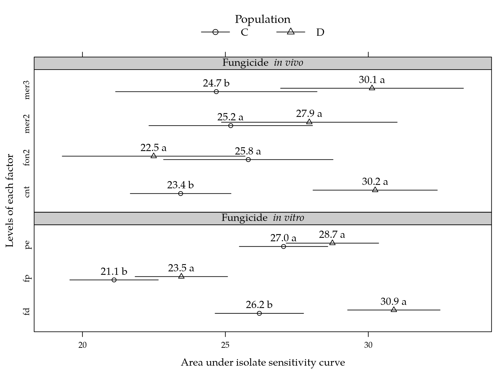
Figure 7: Area under isolate sensitivity curve for combination between population and in vitro fungicide (top) and population and in vivo fungicide (bottom). Pairs of means comparing populations in each row of the plot (each factor level at the y-axis) followed by the same letter are not statistically different at 5% significance level.
Session information
## quinta, 11 de julho de 2019, 20:04
## ----------------------------------------
## R version 3.6.1 (2019-07-05)
## Platform: x86_64-pc-linux-gnu (64-bit)
## Running under: Ubuntu 18.04.2 LTS
##
## Matrix products: default
## BLAS:   /usr/lib/x86_64-linux-gnu/blas/libblas.so.3.7.1
## LAPACK: /usr/lib/x86_64-linux-gnu/lapack/liblapack.so.3.7.1
##
## locale:
##  [1] LC_CTYPE=pt_BR.UTF-8       LC_NUMERIC=C
##  [3] LC_TIME=pt_BR.UTF-8        LC_COLLATE=en_US.UTF-8
##  [5] LC_MONETARY=pt_BR.UTF-8    LC_MESSAGES=en_US.UTF-8
##  [7] LC_PAPER=pt_BR.UTF-8       LC_NAME=C
##  [9] LC_ADDRESS=C               LC_TELEPHONE=C
## [11] LC_MEASUREMENT=pt_BR.UTF-8 LC_IDENTIFICATION=C
##
## attached base packages:
## [1] splines   stats     graphics  grDevices utils     datasets
## [7] methods   base
##
## other attached packages:
##  [1] captioner_2.2.3     knitr_1.23          RDASC_0.0-6
##  [4] wzRfun_0.81         multcomp_1.4-10     TH.data_1.0-10
##  [7] MASS_7.3-51.4       survival_2.44-1.1   mvtnorm_1.0-11
## [10] doBy_4.6-2          lmerTest_3.1-0      lme4_1.1-21
## [13] Matrix_1.2-17       plyr_1.8.4          latticeExtra_0.6-28
## [16] RColorBrewer_1.1-2  lattice_0.20-38
##
## loaded via a namespace (and not attached):
##  [1] zoo_1.8-6           tidyselect_0.2.5    xfun_0.8
##  [4] purrr_0.3.2         tcltk_3.6.1         colorspace_1.4-1
##  [7] htmltools_0.3.6     rpanel_1.1-4        yaml_2.2.0
## [10] rlang_0.4.0         pkgdown_1.3.0       nloptr_1.2.1
## [13] pillar_1.4.2        glue_1.3.1          stringr_1.4.0
## [16] munsell_0.5.0       commonmark_1.7      gtable_0.3.0
## [19] codetools_0.2-16    memoise_1.1.0       evaluate_0.14
## [22] parallel_3.6.1      pbkrtest_0.4-7      highr_0.8
## [25] Rcpp_1.0.1          scales_1.0.0        backports_1.1.4
## [28] desc_1.2.0          fs_1.3.1            ggplot2_3.2.0
## [31] digest_0.6.20       stringi_1.4.3       dplyr_0.8.3
## [34] numDeriv_2016.8-1.1 grid_3.6.1          rprojroot_1.3-2
## [37] tools_3.6.1         sandwich_2.5-1      magrittr_1.5
## [40] lazyeval_0.2.2      tibble_2.1.3        crayon_1.3.4
## [43] pkgconfig_2.0.2     xml2_1.2.0          assertthat_0.2.1
## [46] minqa_1.2.4         rmarkdown_1.13      roxygen2_6.1.1
## [49] R6_2.4.0            boot_1.3-23         nlme_3.1-140
## [52] compiler_3.6.1