Número de Flores de Dendezeiro
Gustavo Azevedo Campos, Rosiana Rodrigues Alves & Walmes Zeviani
2019-07-11
elaeis_flowers.RmdDefinições da Sessão
#-----------------------------------------------------------------------
# Carregando pacotes e funções necessárias.

# https://github.com/walmes/wzRfun
# devtools::install_github("walmes/wzRfun")
library(wzRfun)
library(lattice)
library(latticeExtra)
library(doBy)
library(multcomp)library(RDASC)Análise Exploratória
#-----------------------------------------------------------------------
# Estrutura dos dados.

data(elaeis_flowers)

# Nome curto para agilizar a digitação.
ela <- elaeis_flowers
str(ela)
## 'data.frame': 611 obs. of 8 variables:
## $ cult : Factor w/ 4 levels "1001","2301",..: 1 1 1 2 2 2 3 3 3 4 ...
## $ bloc : Factor w/ 4 levels "B1","B2","B3",..: 1 1 1 1 1 1 1 1 1 1 ...
## $ plant : int 1 2 3 1 2 3 1 2 3 1 ...
## $ days : int 1 1 1 1 1 1 1 1 1 1 ...
## $ tot : int 0 0 0 0 0 0 0 0 2 0 ...
## $ female: int 0 0 0 0 0 0 0 0 2 0 ...
## $ male : int 0 0 0 0 0 0 0 0 0 0 ...
## $ abort : int NA NA NA NA NA NA NA NA NA NA ...ela$ue <- with(ela,
interaction(cult, bloc, plant,
drop = TRUE))
levels(ela$ue) <- 1:nlevels(ela$ue)
L <- list(columns = 4, title = "Blocos", cex.title = 1.1)
xyplot(tot ~ days | cult,
groups = bloc,
data = ela,
type = c("p", "a"),
auto.key = L,
ylab = "Total de flores",
xlab = "Dias")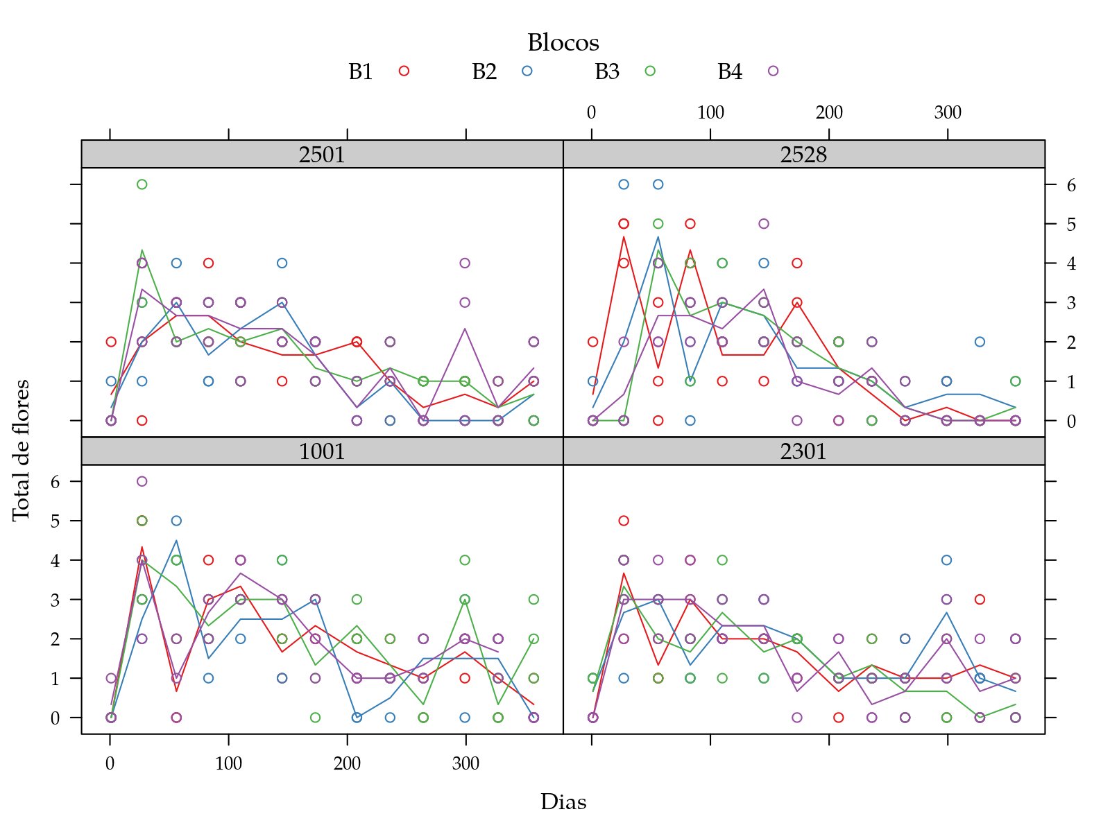
xyplot(male + female ~ days | ue,
       data = ela,
       type = "o",
       auto.key = TRUE,
       as.table = TRUE,
       strip = FALSE,
       ylab = "Total de flores",
       xlab = "Dias")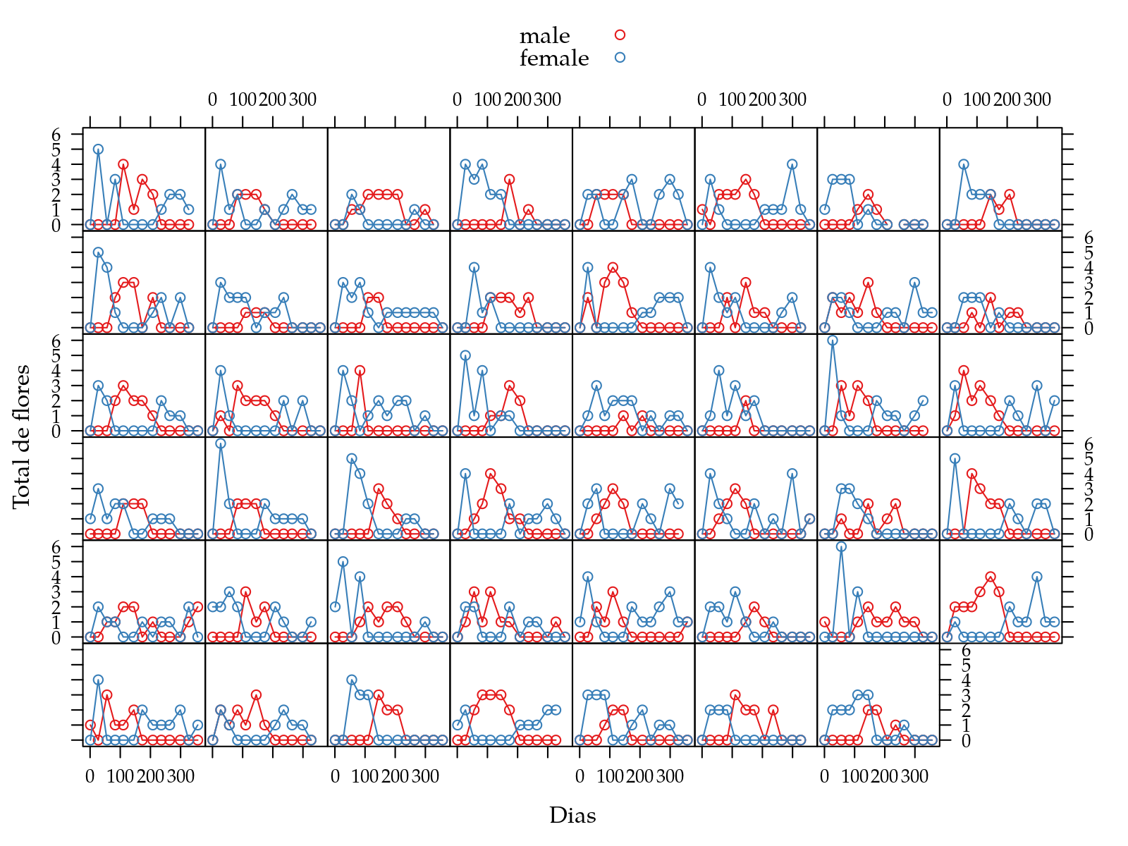
xyplot(abort ~ days | cult,
       groups = bloc,
       data = ela,
       type = c("p", "a"),
       auto.key = L,
       ylab = "Total de flores",
       xlab = "Dias")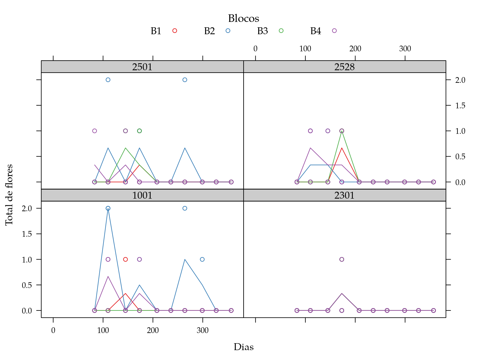
xyplot(female/tot ~ days | cult,
       groups = bloc,
       data = ela,
       type = c("p", "a"),
       auto.key = L,
       ylab = "Total de flores",
       xlab = "Dias")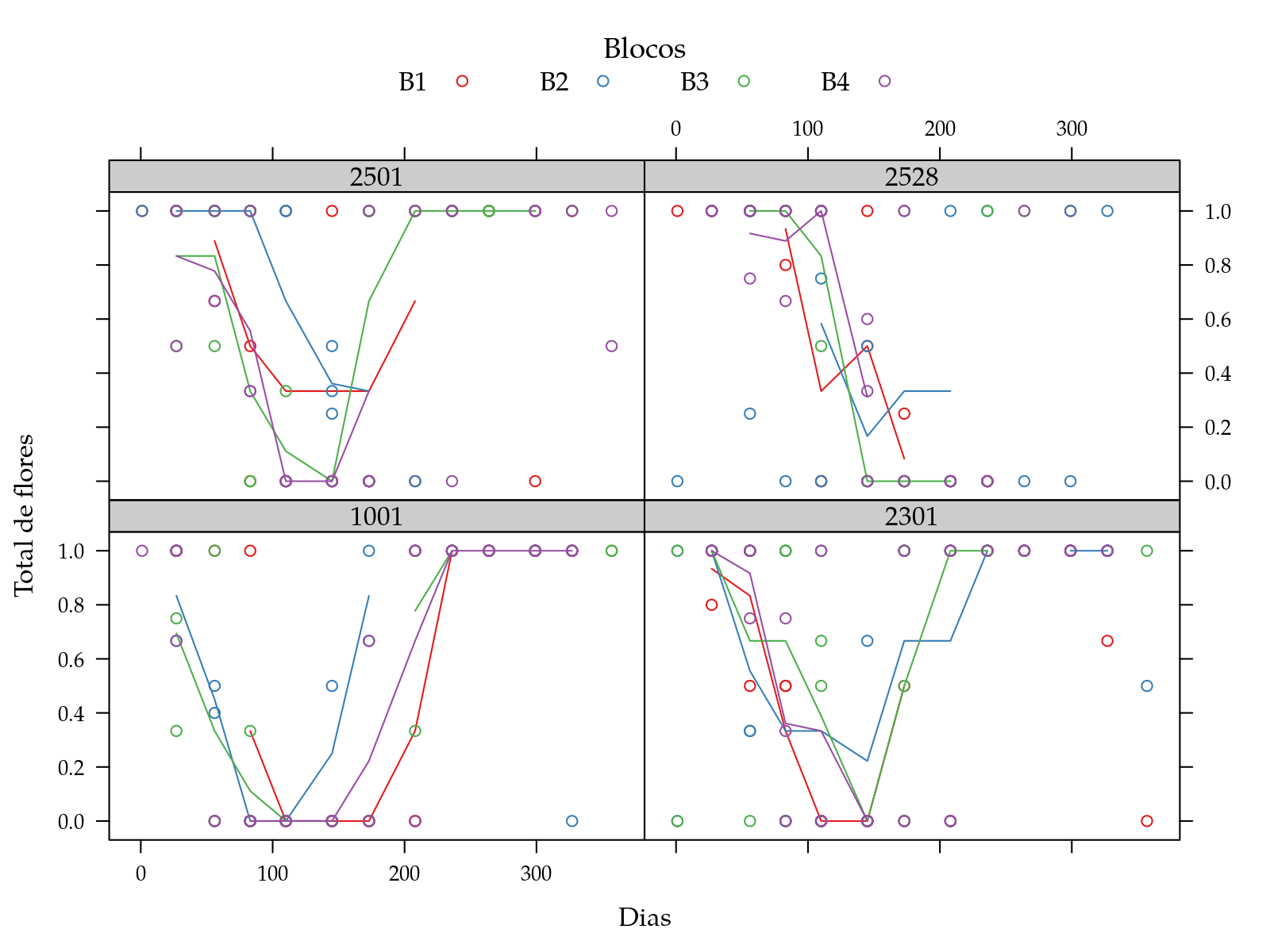
Número Total de Flores
#-----------------------------------------------------------------------
# Ajuste do modelo GLM Poisson.

m0 <- glm(tot ~ bloc + cult * poly(days, deggre = 1),
          data = ela2,
          family = poisson)

# Resíduos.
par(mfrow = c(2, 2))
plot(m0)
##
## Call:
## glm(formula = tot ~ bloc + cult * poly(days, deggre = 1), family = poisson,
##     data = ela2)
##
## Deviance Residuals:
##     Min       1Q   Median       3Q      Max
## -2.8007  -0.9154  -0.1194   0.5501   2.9716
##
## Coefficients:
##                                 Estimate Std. Error z value
## (Intercept)                      1.51567    0.10280  14.744
## blocB2                          -0.20719    0.11420  -1.814
## blocB3                          -0.02367    0.10879  -0.218
## blocB4                           0.01739    0.10768   0.162
## cult2301                        -0.12322    0.11545  -1.067
## cult2501                        -0.37861    0.12772  -2.964
## cult2528                        -0.54744    0.14027  -3.903
## poly(days, deggre = 1)          -5.30733    0.96718  -5.487
## cult2301:poly(days, deggre = 1)  0.01668    1.41189   0.012
## cult2501:poly(days, deggre = 1) -2.99376    1.52579  -1.962
## cult2528:poly(days, deggre = 1) -6.38391    1.61904  -3.943
##                                 Pr(>|z|)
## (Intercept)                      < 2e-16 ***
## blocB2                           0.06964 .
## blocB3                           0.82777
## blocB4                           0.87169
## cult2301                         0.28585
## cult2501                         0.00303 **
## cult2528                        9.51e-05 ***
## poly(days, deggre = 1)          4.08e-08 ***
## cult2301:poly(days, deggre = 1)  0.99058
## cult2501:poly(days, deggre = 1)  0.04975 *
## cult2528:poly(days, deggre = 1) 8.05e-05 ***
## ---
## Signif. codes:  0 '***' 0.001 '**' 0.01 '*' 0.05 '.' 0.1 ' ' 1
##
## (Dispersion parameter for poisson family taken to be 1)
##
##     Null deviance: 410.19  on 159  degrees of freedom
## Residual deviance: 181.12  on 149  degrees of freedom
## AIC: 649.52
##
## Number of Fisher Scoring iterations: 5
# Quadro de Deviance.
anova(m0, test = "Chisq")## Analysis of Deviance Table
##
## Model: poisson, link: log
##
## Response: tot
##
## Terms added sequentially (first to last)
##
##
## Df Deviance Resid. Df Resid. Dev
## NULL 159 410.19
## bloc 3 4.930 156 405.26
## cult 3 7.115 153 398.15
## poly(days, deggre = 1) 1 195.853 152 202.29
## cult:poly(days, deggre = 1) 3 21.176 149 181.12
## Pr(>Chi)
## NULL
## bloc 0.17703
## cult 0.06832 .
## poly(days, deggre = 1) < 2.2e-16 ***
## cult:poly(days, deggre = 1) 9.678e-05 ***
## ---
## Signif. codes: 0 '***' 0.001 '**' 0.01 '*' 0.05 '.' 0.1 ' ' 1# Predição.
pred <- with(ela,
expand.grid(bloc = levels(bloc)[1],
cult = levels(cult),
days = seq(min(days), max(days), by = 2)))
pred$y <- predict(m0, newdata = pred, type = "response")
xyplot(tot ~ days | cult,
data = ela2,
ylab = "Total de flores",
xlab = "Dias") +
as.layer(xyplot(y ~ days | cult, data = pred, type = "l"))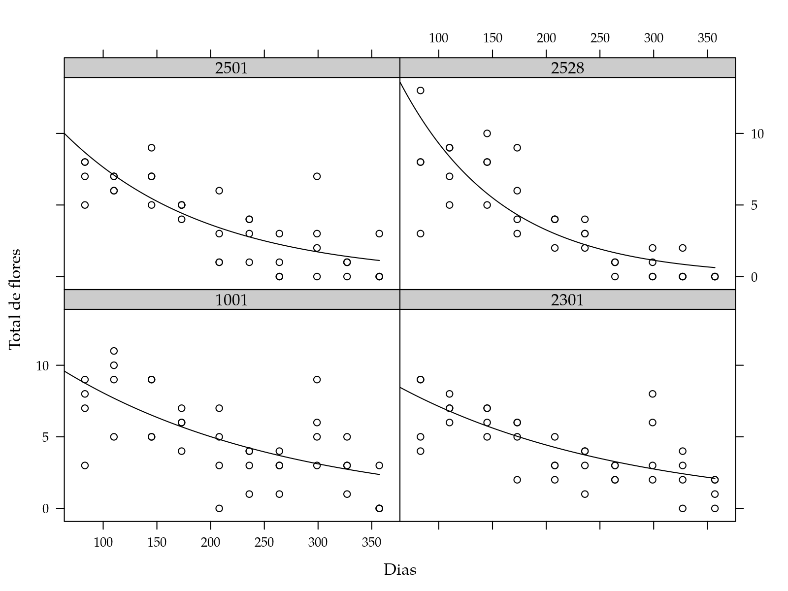
Proporção de Flores Fêmeas
#-----------------------------------------------------------------------
# Ajuste do modelo GLM Binomial.

m0 <- glm(cbind(female, tot - female) ~
              bloc + cult * poly(days, deggre = 2),
          data = ela2,
          family = quasibinomial)

# Resíduos.
par(mfrow = c(2, 2))
plot(m0)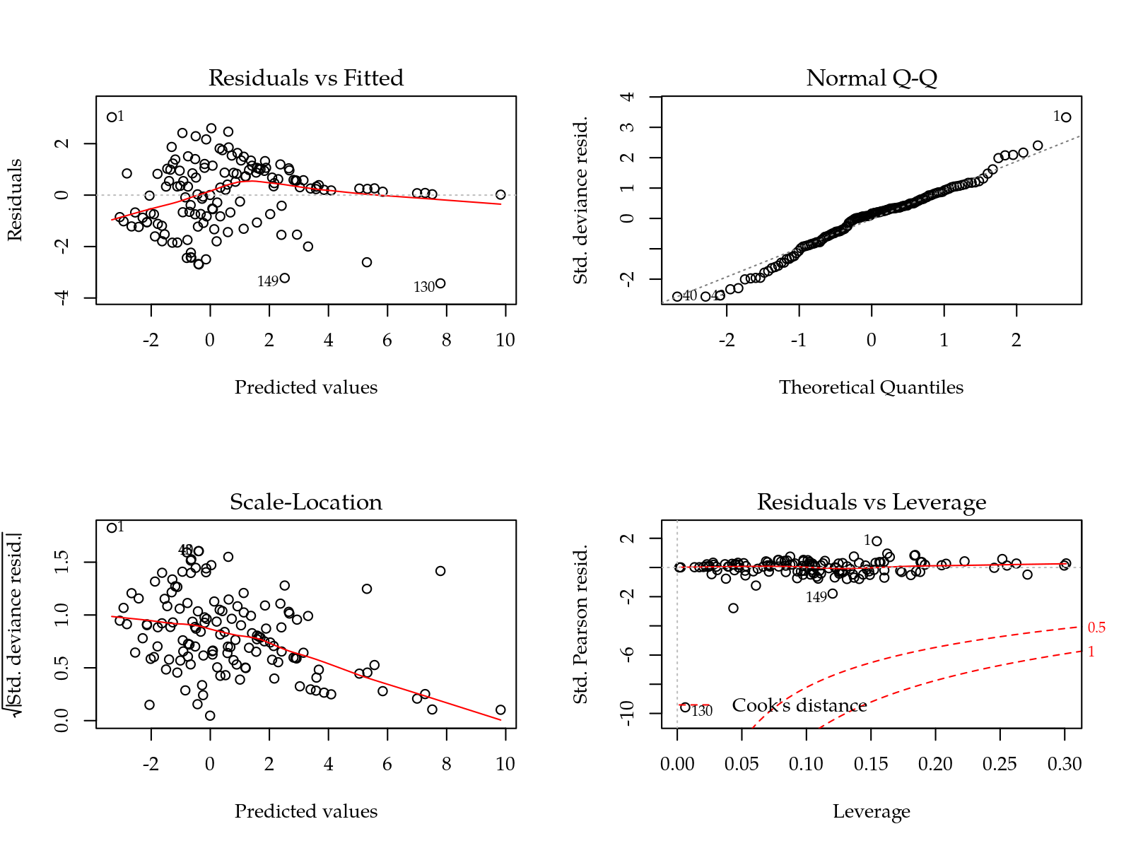
##
## Call:
## glm(formula = cbind(female, tot - female) ~ bloc + cult * poly(days,
##     deggre = 2), family = quasibinomial, data = ela2)
##
## Deviance Residuals:
##     Min       1Q   Median       3Q      Max
## -3.4302  -0.7351   0.0113   0.8443   3.0299
##
## Coefficients:
##                                  Estimate Std. Error t value
## (Intercept)                        1.5989     2.4658   0.648
## blocB2                             0.7913     0.8588   0.921
## blocB3                             0.5124     0.8298   0.617
## blocB4                             0.2711     0.8365   0.324
## cult2301                          -1.1492     2.5463  -0.451
## cult2501                          -0.6880     2.7626  -0.249
## cult2528                          -1.2984     2.8988  -0.448
## poly(days, deggre = 2)1           51.2887    34.4499   1.489
## poly(days, deggre = 2)2           10.9150    22.9166   0.476
## cult2301:poly(days, deggre = 2)1 -35.1421    36.0391  -0.975
## cult2501:poly(days, deggre = 2)1 -27.8811    39.5414  -0.705
## cult2528:poly(days, deggre = 2)1 -37.8795    41.1640  -0.920
## cult2301:poly(days, deggre = 2)2 -10.2569    24.5954  -0.417
## cult2501:poly(days, deggre = 2)2  -1.3348    26.1069  -0.051
## cult2528:poly(days, deggre = 2)2  16.6141    27.9418   0.595
##                                  Pr(>|t|)
## (Intercept)                         0.518
## blocB2                              0.359
## blocB3                              0.538
## blocB4                              0.746
## cult2301                            0.653
## cult2501                            0.804
## cult2528                            0.655
## poly(days, deggre = 2)1             0.139
## poly(days, deggre = 2)2             0.635
## cult2301:poly(days, deggre = 2)1    0.331
## cult2501:poly(days, deggre = 2)1    0.482
## cult2528:poly(days, deggre = 2)1    0.359
## cult2301:poly(days, deggre = 2)2    0.677
## cult2501:poly(days, deggre = 2)2    0.959
## cult2528:poly(days, deggre = 2)2    0.553
##
## (Dispersion parameter for quasibinomial family taken to be 8.820417)
##
##     Null deviance: 517.49  on 136  degrees of freedom
## Residual deviance: 229.63  on 122  degrees of freedom
## AIC: NA
##
## Number of Fisher Scoring iterations: 7
# Quadro de Deviance.
anova(m0, test = "F")## Analysis of Deviance Table
##
## Model: quasibinomial, link: logit
##
## Response: cbind(female, tot - female)
##
## Terms added sequentially (first to last)
##
##
## Df Deviance Resid. Df Resid. Dev F
## NULL 136 517.49
## bloc 3 5.423 133 512.07 0.2050
## cult 3 4.526 130 507.54 0.1710
## poly(days, deggre = 2) 2 151.563 128 355.98 8.5916
## cult:poly(days, deggre = 2) 6 126.354 122 229.63 2.3875
## Pr(>F)
## NULL
## bloc 0.892803
## cult 0.915783
## poly(days, deggre = 2) 0.000323 ***
## cult:poly(days, deggre = 2) 0.032393 *
## ---
## Signif. codes: 0 '***' 0.001 '**' 0.01 '*' 0.05 '.' 0.1 ' ' 1# Predição.
pred <- with(ela,
expand.grid(bloc = levels(bloc)[1],
cult = levels(cult),
days = seq(min(days), max(days), by = 2)))
pred$y <- predict(m0, newdata = pred, type = "response")
xyplot(female/tot ~ days | cult,
data = ela2,
ylab = "Proporção de flores fêmeas",
xlab = "Dias") +
as.layer(xyplot(y ~ days | cult, data = pred, type = "l"))
library(mgcv)

m0 <- gam(cbind(female, tot - female) ~ bloc + s(days, by = cult),
          data = ela2,
          family = quasibinomial)

# plot(m0, pages = 1, residuals = TRUE)
plot(m0, pages = 1, seWithMean = TRUE)
summary(m0)##
## Family: quasibinomial
## Link function: logit
##
## Formula:
## cbind(female, tot - female) ~ bloc + s(days, by = cult)
##
## Parametric coefficients:
## Estimate Std. Error t value Pr(>|t|)
## (Intercept) 0.4438 0.2997 1.481 0.14099
## blocB2 1.0536 0.3606 2.922 0.00406 **
## blocB3 0.6203 0.3464 1.791 0.07552 .
## blocB4 0.3507 0.3481 1.008 0.31544
## ---
## Signif. codes: 0 '***' 0.001 '**' 0.01 '*' 0.05 '.' 0.1 ' ' 1
##
## Approximate significance of smooth terms:
## edf Ref.df F p-value
## s(days):cult1001 5.731 6.809 8.406 1.84e-08 ***
## s(days):cult2301 5.434 6.467 6.244 3.74e-06 ***
## s(days):cult2501 3.727 4.607 7.139 1.21e-05 ***
## s(days):cult2528 3.019 3.734 12.127 4.68e-08 ***
## ---
## Signif. codes: 0 '***' 0.001 '**' 0.01 '*' 0.05 '.' 0.1 ' ' 1
##
## R-sq.(adj) = 0.759 Deviance explained = 71.6%
## GCV = 1.2312 Scale est. = 1.3373 n = 160anova(m0)##
## Family: quasibinomial
## Link function: logit
##
## Formula:
## cbind(female, tot - female) ~ bloc + s(days, by = cult)
##
## Parametric Terms:
## df F p-value
## bloc 3 3.048 0.0309
##
## Approximate significance of smooth terms:
## edf Ref.df F p-value
## s(days):cult1001 5.731 6.809 8.406 1.84e-08
## s(days):cult2301 5.434 6.467 6.244 3.74e-06
## s(days):cult2501 3.727 4.607 7.139 1.21e-05
## s(days):cult2528 3.019 3.734 12.127 4.68e-08# # Resíduos.
# par(mfrow = c(2, 2))
# qqnorm(residuals(m0, type = "pearson"))
# layout(1)
pred <- with(ela,
expand.grid(bloc = levels(bloc)[1],
cult = levels(cult),
days = seq(min(days), max(days), by = 2)))
pred$y <- predict(m0, newdata = pred, type = "response")
xyplot(female/tot ~ days | cult,
data = ela2,
ylab = "Proporção de flores fêmeas",
xlab = "Dias") +
as.layer(xyplot(y ~ days | cult, data = pred, type = "l"))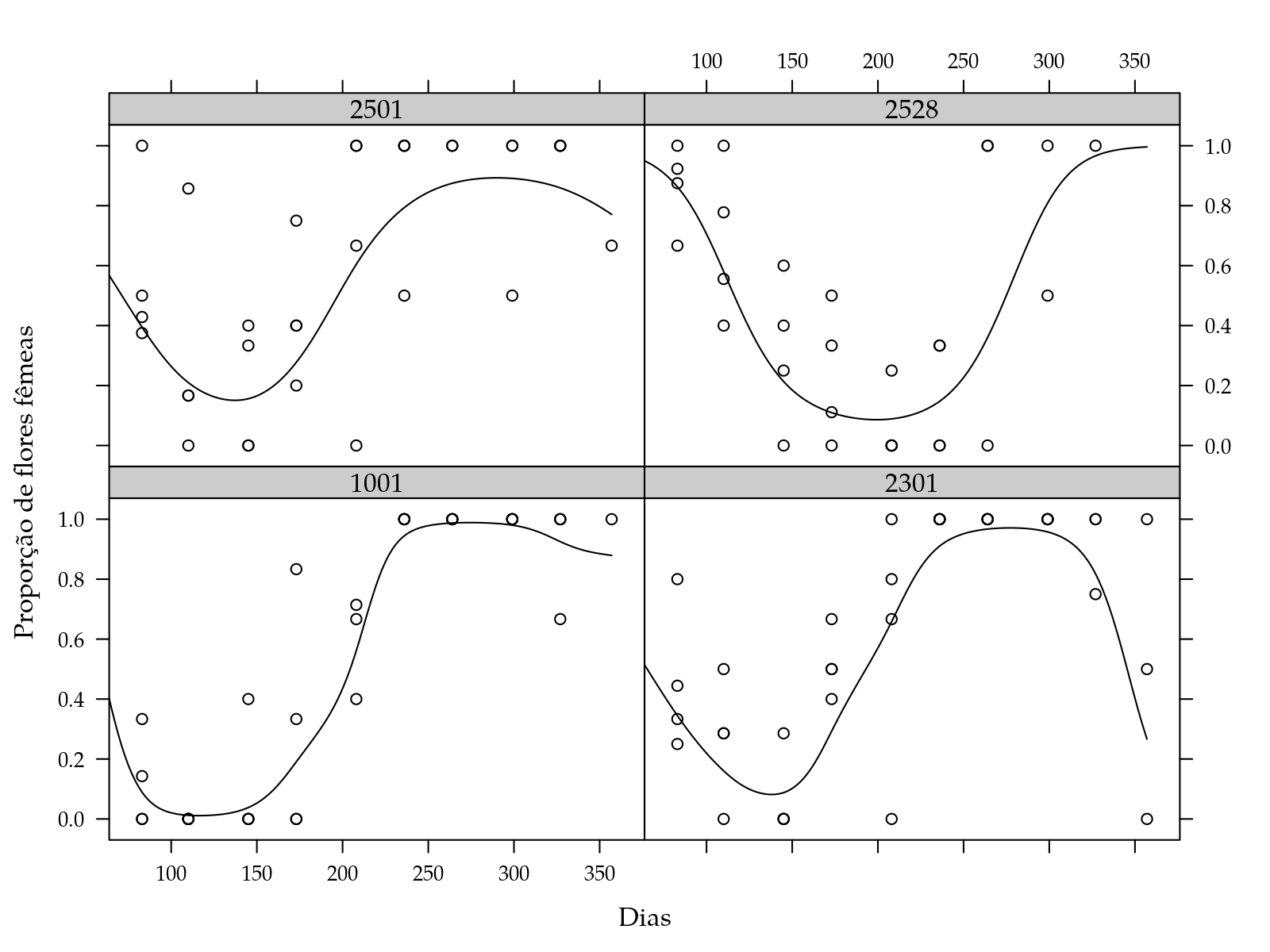
Session information
## quinta, 11 de julho de 2019, 20:05
## ----------------------------------------
## R version 3.6.1 (2019-07-05)
## Platform: x86_64-pc-linux-gnu (64-bit)
## Running under: Ubuntu 18.04.2 LTS
##
## Matrix products: default
## BLAS:   /usr/lib/x86_64-linux-gnu/blas/libblas.so.3.7.1
## LAPACK: /usr/lib/x86_64-linux-gnu/lapack/liblapack.so.3.7.1
##
## locale:
##  [1] LC_CTYPE=pt_BR.UTF-8       LC_NUMERIC=C
##  [3] LC_TIME=pt_BR.UTF-8        LC_COLLATE=en_US.UTF-8
##  [5] LC_MONETARY=pt_BR.UTF-8    LC_MESSAGES=en_US.UTF-8
##  [7] LC_PAPER=pt_BR.UTF-8       LC_NAME=C
##  [9] LC_ADDRESS=C               LC_TELEPHONE=C
## [11] LC_MEASUREMENT=pt_BR.UTF-8 LC_IDENTIFICATION=C
##
## attached base packages:
## [1] stats     graphics  grDevices utils     datasets  methods
## [7] base
##
## other attached packages:
##  [1] mgcv_1.8-28         nlme_3.1-140        captioner_2.2.3
##  [4] knitr_1.23          RDASC_0.0-6         multcomp_1.4-10
##  [7] TH.data_1.0-10      MASS_7.3-51.4       survival_2.44-1.1
## [10] mvtnorm_1.0-11      doBy_4.6-2          latticeExtra_0.6-28
## [13] RColorBrewer_1.1-2  lattice_0.20-38     wzRfun_0.81
##
## loaded via a namespace (and not attached):
##  [1] Rcpp_1.0.1       compiler_3.6.1   pillar_1.4.2
##  [4] plyr_1.8.4       tools_3.6.1      digest_0.6.20
##  [7] evaluate_0.14    memoise_1.1.0    tibble_2.1.3
## [10] pkgconfig_2.0.2  rlang_0.4.0      Matrix_1.2-17
## [13] commonmark_1.7   rpanel_1.1-4     yaml_2.2.0
## [16] pkgdown_1.3.0    xfun_0.8         stringr_1.4.0
## [19] dplyr_0.8.3      roxygen2_6.1.1   xml2_1.2.0
## [22] desc_1.2.0       fs_1.3.1         rprojroot_1.3-2
## [25] grid_3.6.1       tidyselect_0.2.5 glue_1.3.1
## [28] R6_2.4.0         tcltk_3.6.1      rmarkdown_1.13
## [31] purrr_0.3.2      magrittr_1.5     codetools_0.2-16
## [34] splines_3.6.1    backports_1.1.4  htmltools_0.3.6
## [37] assertthat_0.2.1 sandwich_2.5-1   stringi_1.4.3
## [40] crayon_1.3.4     zoo_1.8-6