Desempenho agronômico de milho tratado com bioestimulantes
Tárik Cazeiro El Kadri & Walmes M. Zeviani
11 de julho de 2019
Source:vignettes/bioest_corn.Rmd
bioest_corn.RmdDescrição e Análise Exploratória
#-----------------------------------------------------------------------
# Carrega os pacotes necessários.

rm(list = ls())
library(lattice)
library(latticeExtra)
library(doBy)
library(multcomp)
library(wzRfun)
library(EACS)

#-----------------------------------------------------------------------
# Funções.

# Função para obter a matriz de contrastes pelos índices (li).
contr <- function(li, L) {
    #' @param li Lista com dois elementos onde cada um é um conjunto de
    #'     índices da matriz \code{L}.
    #' @param L Matriz proveniente da função \code{LSmeans()$L} ou
    #'      \code{LE_matrix}.
    #' @return Retorna uma matriz de contrastes de uma linha.
    stopifnot(length(li) == 2L)
    li <- lapply(li,
                 function(i) {
                     if (length(i) == 1) i <- c(i, i) else i
                 })
    l <- lapply(li, function(i) colMeans(L[i, ]))
    k <- rbind(Reduce("-", l))
    if (!is.null(names(li))) {
        rownames(k) <- paste(names(li), collapse = " x ")
    }
    return(k)
}

# Função para obter o intervalo de confiança a partir de um modelo e uma
# matriz de funções lineares.
ic <- function(L, model) {
    conf <- confint(glht(model, linfct = L),
                    calpha = univariate_calpha())$confint
    conf <- as.data.frame(conf)
    if (!is.null(rownames(L))) {
        r <- rownames(L)
        g <- factor(r, levels = r[order(conf[, 1])])
        conf <- cbind(data.frame(contr = g, conf))
    }
    return(conf)
}
O experimento foi realizado para estudar o efeito de bioestimulantes na produção de milho safrinha. Foram estudados 3 fatores descritos a seguir.
-
base: Adubação NPK de base com 3 níveis:0– representa sem adubação de base;NK– representa adubação feita com mistura de uréia e cloreto de potássio, fornecendo portanto apenas N e K;NPK– representa a adubação feita com formulação de fertilizante que contém N, P e K. -
Pe: Uso ou não de P energetic (bioestimulante mineral) como complemento à adubação de base. -
Bk: Uso ou não de Bokashi (bioestimulante orgânico) como complmento à adubação de base.
Dos 3 fatores acima descritos, foram estudadas 10 das 12 possíveis combinações entre os seus níveis, portanto, configurando um experimento em arranjo fatorial triplo incompleto \(3 \times 2 \times 2 - 2 = 10\).
A análise dos resultados, após obtenção da análise de variância e verificação dos pressupostos, será por contrastes planejados. Dois conjuntos de contrastes foram elaborados para serem aplicados ao caso em que houver interação entre os fatores (Tabela 1) e o caso em que apenas for verificado efeitos aditivos (Tabela 2).
| Combinação | I1 | I2 | I3 | I4 | I5 | I6 | I7 | I8 | I9 |
|---|---|---|---|---|---|---|---|---|---|
| NPK | 1/4 | -1 | |||||||
| NPK+Pe | 1/4 | 1/3 | -1/2 | -1/2 | |||||
| NPK+Bk | 1/4 | 1/3 | -1/2 | 1/2 | |||||
| NPK+Pe+Bk | 1/4 | 1/3 | 1 | ||||||
| NK | 1/2 | -1 | |||||||
| NK+Pe | 1/2 | 1 | |||||||
| 0 | -1/4 | -1/4 | -1 | ||||||
| 0+Pe | -1/4 | -1/4 | 1/3 | -1/2 | -1/2 | ||||
| 0+Bk | -1/4 | -1/4 | 1/3 | -1/2 | 1/2 | ||||
| 0+Pe+Bk | -1/4 | -1/4 | 1/3 | 1 |
| Combinação | II1 | II2 | II3 | II4 |
|---|---|---|---|---|
| NPK | 1/4 | -1/2 | ||
| NPK+Pe | 1/4 | 1/6 | 1/2 | |
| NPK+Bk | 1/4 | 1/6 | -1/2 | |
| NPK+Pe+Bk | 1/4 | 1/6 | ||
| NK | 1/2 | |||
| NK+Pe | 1/2 | |||
| 0 | -1/4 | -1/2 | -1/2 | |
| 0+Pe | -1/4 | -1/2 | 1/6 | 1/2 |
| 0+Bk | -1/4 | 1/6 | -1/2 | |
| 0+Pe+Bk | -1/4 | 1/6 |
str(bioest_corn)## 'data.frame': 40 obs. of 8 variables:
## $ bloc: Factor w/ 4 levels "I","II","III",..: 1 1 1 1 1 1 1 1 1 1 ...
## $ adub: Factor w/ 10 levels "NPK","NPK+Pe",..: 1 2 3 4 5 6 7 8 9 10 ...
## $ base: Factor w/ 3 levels "0","NK","NPK": 3 3 3 3 2 2 1 1 1 1 ...
## $ pe : num 0 1 0 1 0 1 0 1 0 1 ...
## $ bk : num 0 0 1 1 0 0 0 0 1 1 ...
## $ prod: num 4306 4761 3094 5417 4006 ...
## $ icol: num 0.471 0.422 0.461 0.471 0.473 ...
## $ m1k : num 28.4 29.8 25.6 29.6 27 ...# Nomes curtos são mais fáceis de manipular.
bio <- bioest_corn
# Número de níveis por cela experimental.
cbind(xtabs(~adub, data = bio))## [,1]
## NPK 4
## NPK+Pe 4
## NPK+Bk 4
## NPK+Pe+Bk 4
## NK 4
## NK+Pe 4
## 0 4
## 0+Pe 4
## 0+Bk 4
## 0+Pe+Bk 4## base 0 NK NPK
## bk pe
## 0 0 4 4 4
## 1 4 4 4
## 1 0 4 0 4
## 1 4 0 4xyplot(prod + icol + m1k ~ adub,
data = bio,
outer = TRUE,
layout = c(NA, 1),
groups = bloc,
type = c("a", "p"),
xlab = "Forma de adubação",
ylab = "Valor da variável resposta",
scales = list(y = list(relation = "free"),
x = list(rot = 90),
alternating = 1)) +
as.layer(xyplot(prod + icol + m1k ~ adub,
data = bio,
type = "a",
col = 1,
lwd = 2))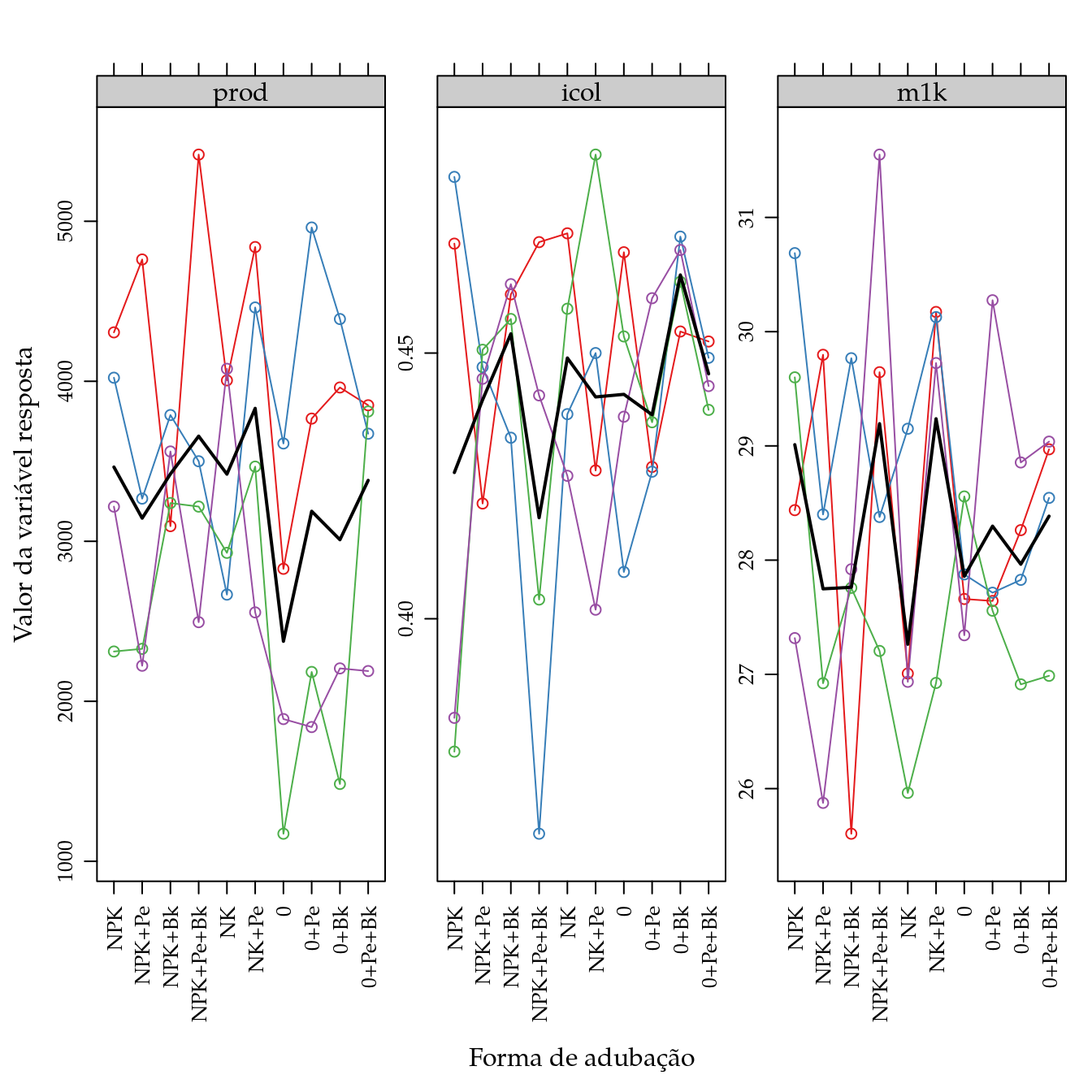
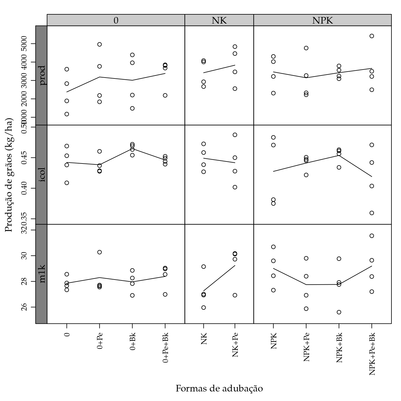
useOuterStrips(
    combineLimits(
        resizePanels(
            xyplot(prod + icol + m1k ~ adub | base,
                   data = bio,
                   outer = TRUE,
                   xlab = "Formas de adubação",
                   ylab = "Produção de grãos (kg/ha)",
                   scales = list(y = list(relation = "free"),
                                 x = list(relation = "free",
                                          rot = 90)),
                   type = c("a", "p")),
            w = c(4, 2, 4))
    )
)
Análise da produção de grãos
#-----------------------------------------------------------------------
# Ajuste do modelo.

# Modelo com um fator de 10 níveis.
m0 <- lm(prod ~ bloc + adub, data = bio)

# Verificação dos pressupostos.
par(mfrow = c(2, 2))
plot(m0)
## Analysis of Variance Table
##
## Response: prod
##           Df   Sum Sq Mean Sq F value    Pr(>F)
## bloc       3 18236491 6078830  10.618 8.703e-05 ***
## adub       9  5786450  642939   1.123    0.3808
## Residuals 27 15457330  572494
## ---
## Signif. codes:  0 '***' 0.001 '**' 0.01 '*' 0.05 '.' 0.1 ' ' 1
#-----------------------------------------------------------------------
# Obtendo as médias para fazer contrastes.
# Médias ajustadas.
lsm <- LSmeans(m0, effect = "adub")
str(lsm)## List of 3
## $ coef:'data.frame': 10 obs. of 5 variables:
## ..$ estimate: num [1:10] 3464 3144 3421 3657 3419 ...
## ..$ se : num [1:10] 378 378 378 378 378 ...
## ..$ df : num [1:10] 27 27 27 27 27 27 27 27 27 27
## ..$ t.stat : num [1:10] 9.16 8.31 9.04 9.67 9.04 ...
## ..$ p.value : num [1:10] 9.09e-10 6.39e-09 1.18e-09 2.93e-10 1.19e-09 ...
## $ grid:'data.frame': 10 obs. of 1 variable:
## ..$ adub: chr [1:10] "NPK" "NPK+Pe" "NPK+Bk" "NPK+Pe+Bk" ...
## $ L : 'LE_matrix_class' num [1:10, 1:13] 1 1 1 1 1 1 1 1 1 1 ...
## ..- attr(*, "dimnames")=List of 2
## .. ..$ : NULL
## .. ..$ : chr [1:13] "(Intercept)" "blocII" "blocIII" "blocIV" ...
## ..- attr(*, "grid")='data.frame': 10 obs. of 1 variable:
## .. ..$ adub: chr [1:10] "NPK" "NPK+Pe" "NPK+Bk" "NPK+Pe+Bk" ...
## - attr(*, "class")= chr "linest_class"# Matriz de coeficientes para obter as ls-means.
L <- lsm$L
# Tabela com o nome dos tratamentos na ordem das médias.
grid <- equallevels(lsm$grid, bio)
rownames(L) <- grid$adub#-----------------------------------------------------------------------
# Contrastes da tabela 1.
# I1.
li <- list("NPK" = 1:4, "0" = 7:10)
K <- contr(li, L)
summary(glht(m0, linfct = K))##
## Simultaneous Tests for General Linear Hypotheses
##
## Fit: lm(formula = prod ~ bloc + adub, data = bio)
##
## Linear Hypotheses:
## Estimate Std. Error t value Pr(>|t|)
## NPK x 0 == 0 433.3 267.5 1.62 0.117
## (Adjusted p values reported -- single-step method)##
## Simultaneous Tests for General Linear Hypotheses
##
## Fit: lm(formula = prod ~ bloc + adub, data = bio)
##
## Linear Hypotheses:
## Estimate Std. Error t value Pr(>|t|)
## NK x 0 == 0 843.8 378.3 2.23 0.0342 *
## ---
## Signif. codes: 0 '***' 0.001 '**' 0.01 '*' 0.05 '.' 0.1 ' ' 1
## (Adjusted p values reported -- single-step method)#--------------------------------------------
# Dentro de sem aduação 0.
# I3.
li <- list("0 | Com+" = 8:10, "Com-" = 7)
K <- contr(li, L)
summary(glht(m0, linfct = K))##
## Simultaneous Tests for General Linear Hypotheses
##
## Fit: lm(formula = prod ~ bloc + adub, data = bio)
##
## Linear Hypotheses:
## Estimate Std. Error t value Pr(>|t|)
## 0 | Com+ x Com- == 0 817.6 436.8 1.872 0.0721 .
## ---
## Signif. codes: 0 '***' 0.001 '**' 0.01 '*' 0.05 '.' 0.1 ' ' 1
## (Adjusted p values reported -- single-step method)##
## Simultaneous Tests for General Linear Hypotheses
##
## Fit: lm(formula = prod ~ bloc + adub, data = bio)
##
## Linear Hypotheses:
## Estimate Std. Error t value Pr(>|t|)
## 0 | Pe + Bk x Pe&Bk == 0 -281.9 463.3 -0.609 0.548
## (Adjusted p values reported -- single-step method)##
## Simultaneous Tests for General Linear Hypotheses
##
## Fit: lm(formula = prod ~ bloc + adub, data = bio)
##
## Linear Hypotheses:
## Estimate Std. Error t value Pr(>|t|)
## 0 | Bk x Pe == 0 -177.8 535.0 -0.332 0.742
## (Adjusted p values reported -- single-step method)#--------------------------------------------
# Dentro de abubação NK.
# I6.
li <- list("NK | Pe+" = 6, "Pe-" = 5)
K <- contr(li, L)
summary(glht(m0, linfct = K))##
## Simultaneous Tests for General Linear Hypotheses
##
## Fit: lm(formula = prod ~ bloc + adub, data = bio)
##
## Linear Hypotheses:
## Estimate Std. Error t value Pr(>|t|)
## NK | Pe+ x Pe- == 0 411.1 535.0 0.768 0.449
## (Adjusted p values reported -- single-step method)#--------------------------------------------
# Dentro de adubação NPK.
# I7.
li <- list("NPK | Com+" = 2:4, "Com-" = 1)
K <- contr(li, L)
summary(glht(m0, linfct = K))##
## Simultaneous Tests for General Linear Hypotheses
##
## Fit: lm(formula = prod ~ bloc + adub, data = bio)
##
## Linear Hypotheses:
## Estimate Std. Error t value Pr(>|t|)
## NPK | Com+ x Com- == 0 -56.49 436.84 -0.129 0.898
## (Adjusted p values reported -- single-step method)# I8.
li <- list("NPK | Pe&Bk" = 4, "Pe + Bk" = 2:3)
K <- contr(li, L)
summary(glht(m0, linfct = K))##
## Simultaneous Tests for General Linear Hypotheses
##
## Fit: lm(formula = prod ~ bloc + adub, data = bio)
##
## Linear Hypotheses:
## Estimate Std. Error t value Pr(>|t|)
## NPK | Pe&Bk x Pe + Bk == 0 374.3 463.3 0.808 0.426
## (Adjusted p values reported -- single-step method)##
## Simultaneous Tests for General Linear Hypotheses
##
## Fit: lm(formula = prod ~ bloc + adub, data = bio)
##
## Linear Hypotheses:
## Estimate Std. Error t value Pr(>|t|)
## NPK | Bk x Pe == 0 276.4 535.0 0.517 0.61
## (Adjusted p values reported -- single-step method)#-----------------------------------------------------------------------
# Contrastes da tabela 2.
# Note que II1 = I1 e II2 = I2. Então já foram feitos.
#--------------------------------------------
# Contrastes sobre a aplicação de Pe e Bk, considerando NPK e 0.
# II3.
li <- list("Com+" = c(2:4, 8:10), "Com-" = c(1, 7))
K <- contr(li, L)
summary(glht(m0, linfct = K))##
## Simultaneous Tests for General Linear Hypotheses
##
## Fit: lm(formula = prod ~ bloc + adub, data = bio)
##
## Linear Hypotheses:
## Estimate Std. Error t value Pr(>|t|)
## Com+ x Com- == 0 380.6 308.9 1.232 0.229
## (Adjusted p values reported -- single-step method)##
## Simultaneous Tests for General Linear Hypotheses
##
## Fit: lm(formula = prod ~ bloc + adub, data = bio)
##
## Linear Hypotheses:
## Estimate Std. Error t value Pr(>|t|)
## Pe x Bk == 0 -49.3 378.3 -0.13 0.897
## (Adjusted p values reported -- single-step method)#-----------------------------------------------------------------------
# Matrizes dos contrastes para o caso de efeitos aditivos e interação.
# Matriz de contrastes quando der interação (9 GL).
li <- list(
list("NPK" = 1:4, "0" = 7:10),
list("NK" = 5:6, "0" = 7:8),
list("0 | Com+" = 8:10, "Com-" = 7),
list("0 | Pe + Bk" = 8:9, "Pe&Bk" = 10),
list("0 | Bk" = 9, "Pe" = 8),
list("NK | Pe+" = 6, "Pe-" = 5),
list("NPK | Com+" = 2:4, "Com-" = 1),
list("NPK | Pe&Bk" = 4, "Pe + Bk" = 2:3),
list("NPK | Bk" = 3, "Pe" = 2))
K <- lapply(li, FUN = contr, L = L)
Ki <- do.call(rbind, K)
summary(glht(m0, linfct = Ki),
test = adjusted(type = "none"))##
## Simultaneous Tests for General Linear Hypotheses
##
## Fit: lm(formula = prod ~ bloc + adub, data = bio)
##
## Linear Hypotheses:
## Estimate Std. Error t value Pr(>|t|)
## NPK x 0 == 0 433.33 267.51 1.620 0.1169
## NK x 0 == 0 843.75 378.32 2.230 0.0342 *
## 0 | Com+ x Com- == 0 817.59 436.84 1.872 0.0721 .
## 0 | Pe + Bk x Pe&Bk == 0 -281.94 463.34 -0.609 0.5479
## 0 | Bk x Pe == 0 -177.78 535.02 -0.332 0.7422
## NK | Pe+ x Pe- == 0 411.11 535.02 0.768 0.4489
## NPK | Com+ x Com- == 0 -56.49 436.84 -0.129 0.8981
## NPK | Pe&Bk x Pe + Bk == 0 374.29 463.34 0.808 0.4263
## NPK | Bk x Pe == 0 276.39 535.02 0.517 0.6096
## ---
## Signif. codes: 0 '***' 0.001 '**' 0.01 '*' 0.05 '.' 0.1 ' ' 1
## (Adjusted p values reported -- none method)# Matriz de contrastes quando não der interação (4 GL).
li <- list(
list("NPK" = 1:4, "0" = 7:10),
list("NK" = 5:6, "0" = 7:8),
list("Com+" = c(2:4, 8:10), "Com-" = c(1, 7)),
list("Pe" = c(2, 8), "Bk" = c(3, 9)))
K <- lapply(li, FUN = contr, L = L)
Ka <- do.call(rbind, K)
summary(glht(m0, linfct = Ka),
test = adjusted(type = "none"))##
## Simultaneous Tests for General Linear Hypotheses
##
## Fit: lm(formula = prod ~ bloc + adub, data = bio)
##
## Linear Hypotheses:
## Estimate Std. Error t value Pr(>|t|)
## NPK x 0 == 0 433.3 267.5 1.620 0.1169
## NK x 0 == 0 843.8 378.3 2.230 0.0342 *
## Com+ x Com- == 0 380.6 308.9 1.232 0.2286
## Pe x Bk == 0 -49.3 378.3 -0.130 0.8973
## ---
## Signif. codes: 0 '***' 0.001 '**' 0.01 '*' 0.05 '.' 0.1 ' ' 1
## (Adjusted p values reported -- none method)#-----------------------------------------------------------------------
# Ajustando os modelos e aplicando os contrastes.
m0 <- lm(prod ~ bloc + adub, data = bio)
# Verificação dos pressupostos.
par(mfrow = c(2, 2))
plot(m0)
layout(1)

# Ajuste do modelo fatorial triplo.
m1 <- update(m0, . ~ bloc + base * pe * bk)

# Modelo reduzido contendo apenas os efeitos principais.
m2 <- update(m0, . ~ bloc + base + pe + bk)

# Teste para hipótese de que os termos abandonados (interações) são
# nulos.
anova(m2, m1)
## Analysis of Variance Table
##
## Model 1: prod ~ bloc + base + pe + bk
## Model 2: prod ~ bloc + base + pe + bk + base:pe + base:bk + pe:bk + base:pe:bk
## Res.Df RSS Df Sum of Sq F Pr(>F)
## 1 32 16857118
## 2 27 15457330 5 1399787 0.489 0.7814anova(m0)## Analysis of Variance Table
##
## Response: prod
## Df Sum Sq Mean Sq F value Pr(>F)
## bloc 3 18236491 6078830 10.618 8.703e-05 ***
## adub 9 5786450 642939 1.123 0.3808
## Residuals 27 15457330 572494
## ---
## Signif. codes: 0 '***' 0.001 '**' 0.01 '*' 0.05 '.' 0.1 ' ' 1anova(m2)## Analysis of Variance Table
##
## Response: prod
## Df Sum Sq Mean Sq F value Pr(>F)
## bloc 3 18236491 6078830 11.5395 2.745e-05 ***
## base 2 2631929 1315964 2.4981 0.09815 .
## pe 1 913363 913363 1.7338 0.19727
## bk 1 841370 841370 1.5972 0.21543
## Residuals 32 16857118 526785
## ---
## Signif. codes: 0 '***' 0.001 '**' 0.01 '*' 0.05 '.' 0.1 ' ' 1# Contrastes para o caso em que não houve interação.
summary(glht(m0, linfct = Ka),
test = adjusted(type = "none"))##
## Simultaneous Tests for General Linear Hypotheses
##
## Fit: lm(formula = prod ~ bloc + adub, data = bio)
##
## Linear Hypotheses:
## Estimate Std. Error t value Pr(>|t|)
## NPK x 0 == 0 433.3 267.5 1.620 0.1169
## NK x 0 == 0 843.8 378.3 2.230 0.0342 *
## Com+ x Com- == 0 380.6 308.9 1.232 0.2286
## Pe x Bk == 0 -49.3 378.3 -0.130 0.8973
## ---
## Signif. codes: 0 '***' 0.001 '**' 0.01 '*' 0.05 '.' 0.1 ' ' 1
## (Adjusted p values reported -- none method)icc <- ic(Ka, m0)
segplot(contr ~ lwr + upr,
centers = Estimate,
data = icc,
draw = FALSE,
xlab = "Estimativa do contraste com IC de 95%",
ylab = "Contraste") +
layer(panel.abline(v = 0, lty = 2)) +
layer(panel.text(x = centers,
y = z,
label = sprintf("%0.3f", centers),
pos = 3))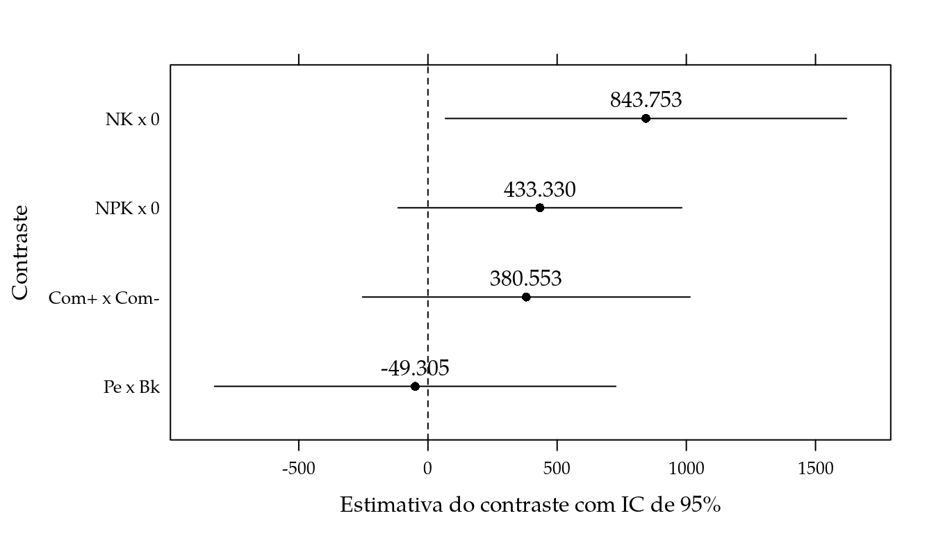
Peso de 1000 grãos
m0 <- lm(m1k ~ bloc + adub, data = bio)

# Verificação dos pressupostos.
par(mfrow = c(2, 2))
plot(m0)
layout(1)

# Ajuste do modelo fatorial triplo.
m1 <- update(m0, . ~ bloc + base * pe * bk)

# Modelo reduzido contendo apenas os efeitos principais.
m2 <- update(m0, . ~ bloc + base + pe + bk)

# Teste para hipótese de que os termos abandonados (interações) são
# nulos.
anova(m2, m1)
## Analysis of Variance Table
##
## Model 1: m1k ~ bloc + base + pe + bk
## Model 2: m1k ~ bloc + base + pe + bk + base:pe + base:bk + pe:bk + base:pe:bk
## Res.Df RSS Df Sum of Sq F Pr(>F)
## 1 32 59.184
## 2 27 46.976 5 12.208 1.4033 0.2546anova(m0)## Analysis of Variance Table
##
## Response: m1k
## Df Sum Sq Mean Sq F value Pr(>F)
## bloc 3 10.721 3.5738 2.0541 0.1299
## adub 9 16.629 1.8477 1.0620 0.4204
## Residuals 27 46.976 1.7399anova(m2)## Analysis of Variance Table
##
## Response: m1k
## Df Sum Sq Mean Sq F value Pr(>F)
## bloc 3 10.721 3.5738 1.9323 0.1442
## base 2 0.738 0.3688 0.1994 0.8202
## pe 1 3.608 3.6075 1.9505 0.1721
## bk 1 0.076 0.0763 0.0413 0.8403
## Residuals 32 59.184 1.8495# Contrastes para o caso em que não houve interação.
summary(glht(m0, linfct = Ka),
test = adjusted(type = "none"))##
## Simultaneous Tests for General Linear Hypotheses
##
## Fit: lm(formula = m1k ~ bloc + adub, data = bio)
##
## Linear Hypotheses:
## Estimate Std. Error t value Pr(>|t|)
## NPK x 0 == 0 0.3027 0.4663 0.649 0.522
## NK x 0 == 0 0.1725 0.6595 0.262 0.796
## Com+ x Com- == 0 -0.2093 0.5385 -0.389 0.701
## Pe x Bk == 0 0.1597 0.6595 0.242 0.811
## (Adjusted p values reported -- none method)icc <- ic(Ka, m0)
segplot(contr ~ lwr + upr,
centers = Estimate,
data = icc,
draw = FALSE,
xlab = "Estimativa do contraste com IC de 95%",
ylab = "Contraste") +
layer(panel.abline(v = 0, lty = 2)) +
layer(panel.text(x = centers,
y = z,
label = sprintf("%0.2f", centers),
pos = 3))
Índice de colheita
m0 <- lm(icol ~ bloc + adub, data = bio)

# Verificação dos pressupostos.
par(mfrow = c(2, 2))
plot(m0)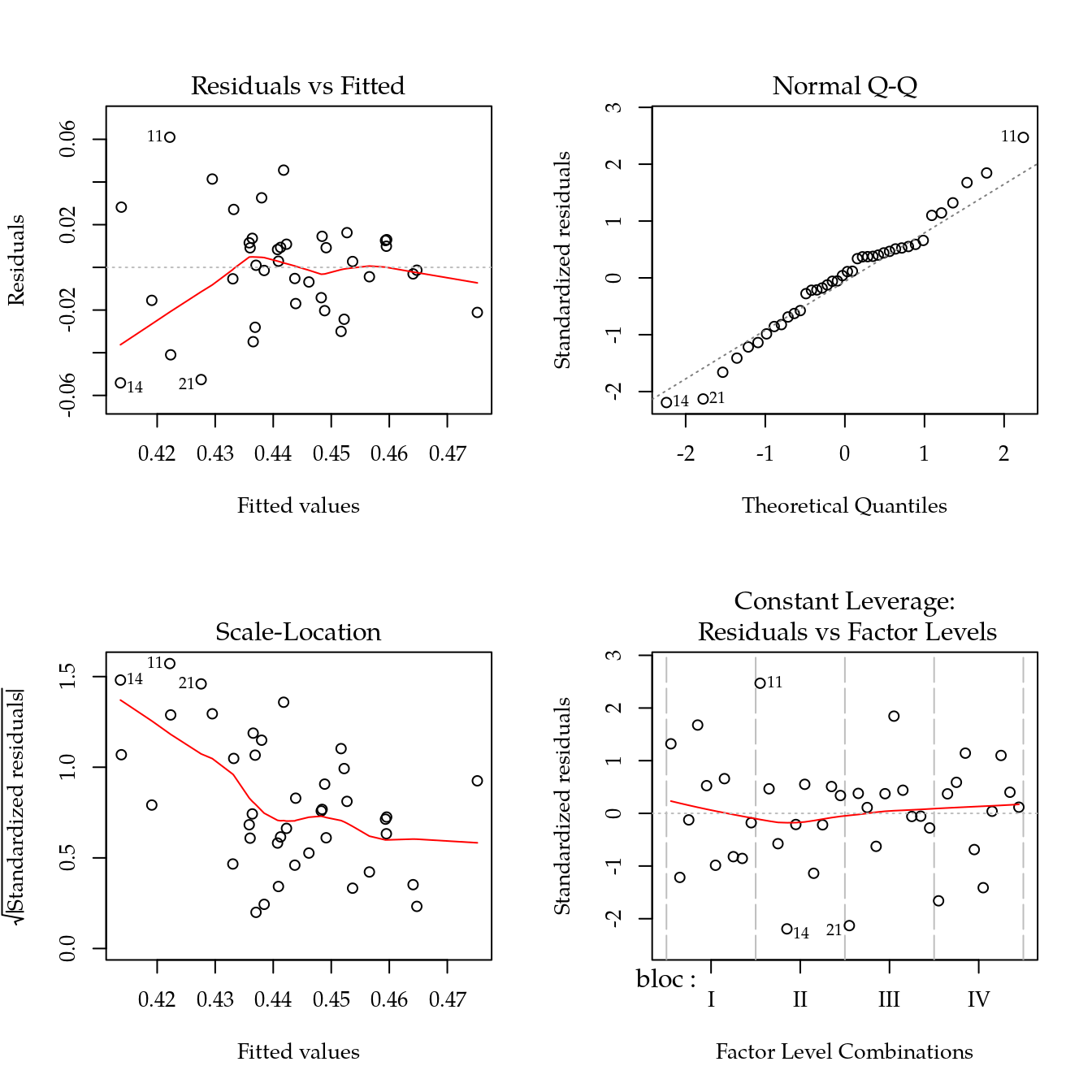
layout(1)

# Ajuste do modelo fatorial triplo.
m1 <- update(m0, . ~ bloc + base * pe * bk)

# Modelo reduzido contendo apenas os efeitos principais.
m2 <- update(m0, . ~ bloc + base + pe + bk)

# Teste para hipótese de que os termos abandonados (interações) são
# nulos.
anova(m2, m1)
## Analysis of Variance Table
##
## Model 1: icol ~ bloc + base + pe + bk
## Model 2: icol ~ bloc + base + pe + bk + base:pe + base:bk + pe:bk + base:pe:bk
## Res.Df RSS Df Sum of Sq F Pr(>F)
## 1 32 0.027277
## 2 27 0.024362 5 0.0029153 0.6462 0.6667anova(m0)## Analysis of Variance Table
##
## Response: icol
## Df Sum Sq Mean Sq F value Pr(>F)
## bloc 3 0.0016541 0.00055138 0.6111 0.6137
## adub 9 0.0058679 0.00065199 0.7226 0.6843
## Residuals 27 0.0243619 0.00090229anova(m2)## Analysis of Variance Table
##
## Response: icol
## Df Sum Sq Mean Sq F value Pr(>F)
## bloc 3 0.0016541 0.00055138 0.6468 0.5907
## base 2 0.0013442 0.00067211 0.7885 0.4632
## pe 1 0.0010277 0.00102767 1.2056 0.2804
## bk 1 0.0005806 0.00058064 0.6812 0.4153
## Residuals 32 0.0272773 0.00085241# Contrastes para o caso em que não houve interação.
summary(glht(m0, linfct = Ka),
test = adjusted(type = "none"))##
## Simultaneous Tests for General Linear Hypotheses
##
## Fit: lm(formula = icol ~ bloc + adub, data = bio)
##
## Linear Hypotheses:
## Estimate Std. Error t value Pr(>|t|)
## NPK x 0 == 0 -0.012507 0.010620 -1.178 0.249
## NK x 0 == 0 0.005097 0.015019 0.339 0.737
## Com+ x Com- == 0 0.008960 0.012263 0.731 0.471
## Pe x Bk == 0 -0.019360 0.015019 -1.289 0.208
## (Adjusted p values reported -- none method)icc <- ic(Ka, m0)
segplot(contr ~ lwr + upr,
centers = Estimate,
data = icc,
draw = FALSE,
xlab = "Estimativa do contraste com IC de 95%",
ylab = "Contraste") +
layer(panel.abline(v = 0, lty = 2)) +
layer(panel.text(x = centers,
y = z,
label = sprintf("%0.3f", centers),
pos = 3))
Informações da Sessão
## Atualizado em 11 de julho de 2019.
##
## R version 3.6.1 (2019-07-05)
## Platform: x86_64-pc-linux-gnu (64-bit)
## Running under: Ubuntu 18.04.2 LTS
##
## Matrix products: default
## BLAS:   /usr/lib/x86_64-linux-gnu/blas/libblas.so.3.7.1
## LAPACK: /usr/lib/x86_64-linux-gnu/lapack/liblapack.so.3.7.1
##
## locale:
##  [1] LC_CTYPE=pt_BR.UTF-8       LC_NUMERIC=C
##  [3] LC_TIME=pt_BR.UTF-8        LC_COLLATE=en_US.UTF-8
##  [5] LC_MONETARY=pt_BR.UTF-8    LC_MESSAGES=en_US.UTF-8
##  [7] LC_PAPER=pt_BR.UTF-8       LC_NAME=C
##  [9] LC_ADDRESS=C               LC_TELEPHONE=C
## [11] LC_MEASUREMENT=pt_BR.UTF-8 LC_IDENTIFICATION=C
##
## attached base packages:
## [1] stats     graphics  grDevices utils     datasets  methods
## [7] base
##
## other attached packages:
##  [1] multcomp_1.4-10     TH.data_1.0-10      MASS_7.3-51.4
##  [4] survival_2.44-1.1   mvtnorm_1.0-11      doBy_4.6-2
##  [7] EACS_0.0-7          wzRfun_0.91         captioner_2.2.3
## [10] latticeExtra_0.6-28 RColorBrewer_1.1-2  lattice_0.20-38
## [13] knitr_1.23
##
## loaded via a namespace (and not attached):
##  [1] zoo_1.8-6         tidyselect_0.2.5  xfun_0.8
##  [4] remotes_2.1.0     purrr_0.3.2       splines_3.6.1
##  [7] testthat_2.1.1    htmltools_0.3.6   usethis_1.5.1
## [10] yaml_2.2.0        rlang_0.4.0       pkgbuild_1.0.3
## [13] pkgdown_1.3.0     pillar_1.4.2      glue_1.3.1
## [16] withr_2.1.2       sessioninfo_1.1.1 plyr_1.8.4
## [19] stringr_1.4.0     commonmark_1.7    devtools_2.1.0
## [22] codetools_0.2-16  memoise_1.1.0     evaluate_0.14
## [25] callr_3.3.0       ps_1.3.0          highr_0.8
## [28] Rcpp_1.0.1        backports_1.1.4   desc_1.2.0
## [31] pkgload_1.0.2     fs_1.3.1          digest_0.6.20
## [34] stringi_1.4.3     processx_3.4.0    dplyr_0.8.3
## [37] grid_3.6.1        rprojroot_1.3-2   cli_1.1.0
## [40] tools_3.6.1       sandwich_2.5-1    magrittr_1.5
## [43] tibble_2.1.3      crayon_1.3.4      pkgconfig_2.0.2
## [46] Matrix_1.2-17     xml2_1.2.0        prettyunits_1.0.2
## [49] assertthat_0.2.1  rmarkdown_1.13    roxygen2_6.1.1
## [52] rstudioapi_0.10   R6_2.4.0          compiler_3.6.1