Resposta de genótipos de pimenta à doses de nitrogênio
Milson E. Serafim & Walmes M. Zeviani
11 de julho de 2019
Source:vignettes/capsicum_nitro.Rmd
capsicum_nitro.RmdDescrição e Análise Exploratória
#-----------------------------------------------------------------------
# Carrega os pacotes necessários.

rm(list = ls())
library(lattice)
library(latticeExtra)
library(plyr)
library(doBy)
library(multcomp)
library(candisc)
library(wzRfun)
library(EACS)## List of 4
## $ cres :'data.frame': 3396 obs. of 5 variables:
## ..$ gen : Factor w/ 8 levels "39 C. chinense",..: 1 1 1 1 1 1 1 1 1 1 ...
## ..$ dose: int [1:3396] 0 1 2 4 8 16 32 64 128 256 ...
## ..$ rept: int [1:3396] 1 1 1 1 1 1 1 1 1 1 ...
## ..$ data: Date[1:3396], format: "2016-06-15" ...
## ..$ alt : int [1:3396] 91 93 82 85 75 95 70 84 76 78 ...
## $ planta:'data.frame': 130 obs. of 9 variables:
## ..$ gen : Factor w/ 8 levels "39 C. chinense",..: 1 1 1 1 1 1 1 1 1 1 ...
## ..$ dose : int [1:130] 0 1 2 4 8 16 32 64 128 256 ...
## ..$ rept : int [1:130] 1 1 1 1 1 1 1 1 1 1 ...
## ..$ flores: int [1:130] 53 35 53 44 53 42 53 53 53 42 ...
## ..$ matur : int [1:130] 149 73 NA NA NA 93 95 86 95 149 ...
## ..$ nfrut : int [1:130] 8 2 NA NA NA 1 1 29 13 13 ...
## ..$ mff : num [1:130] 8.47 8.36 NA NA NA ...
## ..$ msf : num [1:130] 0.98 0.95 NA NA NA ...
## ..$ diamc : num [1:130] 12.33 9.46 8.89 9.3 9.03 ...
## $ fruto :'data.frame': 451 obs. of 6 variables:
## ..$ gen : Factor w/ 8 levels "39 C. chinense",..: 1 1 1 1 1 1 1 1 1 1 ...
## ..$ dose : int [1:451] 0 0 0 0 0 1 1 16 32 64 ...
## ..$ rept : int [1:451] 1 1 1 1 1 1 1 1 1 1 ...
## ..$ fruto: int [1:451] 1 2 3 4 5 1 2 1 1 1 ...
## ..$ diamf: num [1:451] 19 18 23 25 19 27 29 45 46 36 ...
## ..$ compf: num [1:451] 11.9 10.9 14.2 13.5 12.4 ...
## $ teor :'data.frame': 217 obs. of 9 variables:
## ..$ gen : Factor w/ 8 levels "39 C. chinense",..: 1 1 1 1 1 1 1 1 1 1 ...
## ..$ dose : int [1:217] 0 0 0 16 16 16 256 256 256 1 ...
## ..$ rept : int [1:217] 1 1 1 1 1 1 1 1 1 2 ...
## ..$ ddph : num [1:217] 34.4 35.3 34.4 22.3 23.2 ...
## ..$ lico : num [1:217] 0.57 0.48 0.46 0.08 0.38 0.02 NA NA NA 0.06 ...
## ..$ bcaro : num [1:217] 1.35 1.28 1.22 0 0 0.04 NA NA NA 0 ...
## ..$ polifen: num [1:217] 151 154 156 118 106 ...
## ..$ flavon : num [1:217] 35.1 48.7 20.2 NA NA ...
## ..$ antoc : num [1:217] 21.08 19.37 6.51 NA NA ...# Acessa a documentação dos dados.
help(capsicum_nitro, help_type = "html")# Nomes curtos conferem maior agilidade.
cn <- capsicum_nitro
# Para criar uma versão abreviada dos níveis de genótipo.
genab <- function(x){
gsub(pattern = "^(\\d+).*\\s(\\w{3})\\w*$",
replacement = "\\1 \\2",
x)
}
cn <- lapply(cn,
FUN = function(x) {
x$genab <- factor(x$gen,
levels = levels(x$gen),
labels = genab(levels(x$gen)))
return(x)
})
# Versão abreviada dos níveis de genótipo.
sapply(subset(cn$planta, select = c(gen, genab)), FUN = levels)## gen genab
## [1,] "39 C. chinense" "39 chi"
## [2,] "118 C. chinense" "118 chi"
## [3,] "17 C. frutescens" "17 fru"
## [4,] "113 C. frutescens" "113 fru"
## [5,] "116 C. annuun" "116 ann"
## [6,] "163 C. annuun" "163 ann"
## [7,] "66 C. b. var. pendulum" "66 pen"
## [8,] "141 C. b. var. praetermissum" "141 pra"#--------------------------------------------
# Crescimento em altura das plantas.
xyplot(alt ~ data | genab,
groups = interaction(dose, rept),
data = cn$cres,
as.table = TRUE,
layout = c(NA, 2),
type = "l")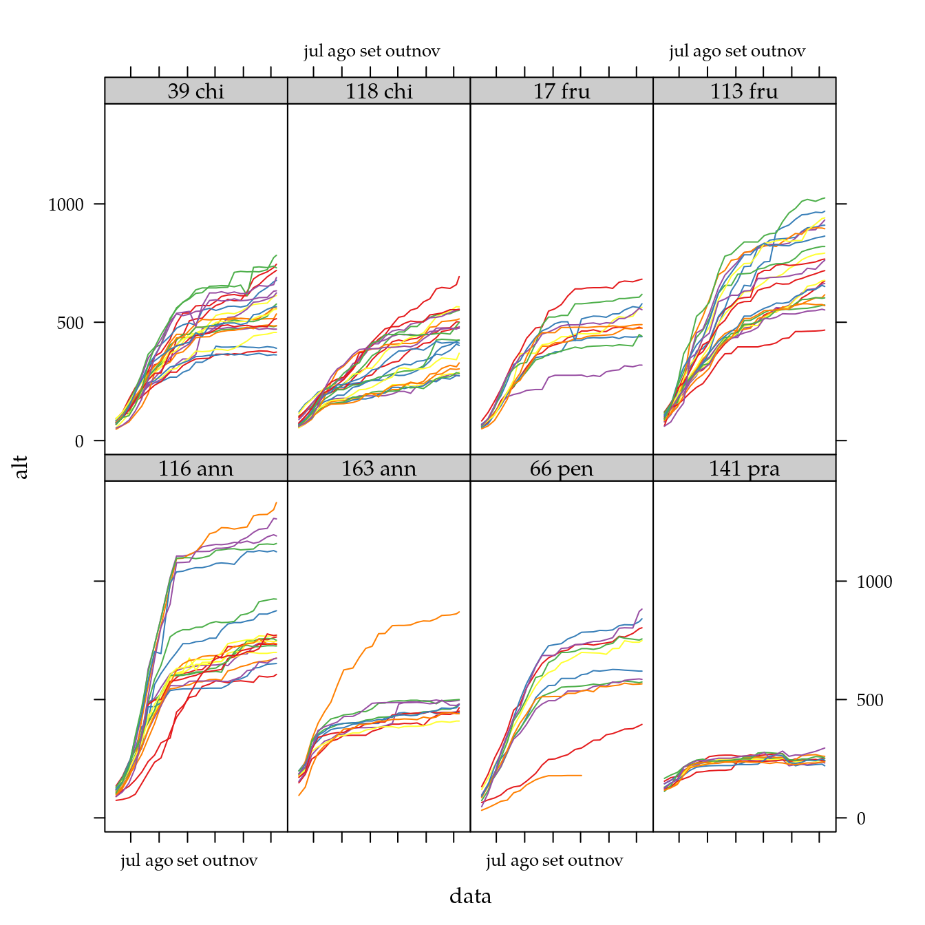
xyplot(alt ~ data | factor(dose),
       groups = genab,
       data = cn$cres,
       as.table = TRUE,
       layout = c(NA, 3),
       auto.key = list(columns = 4),
       type = "a")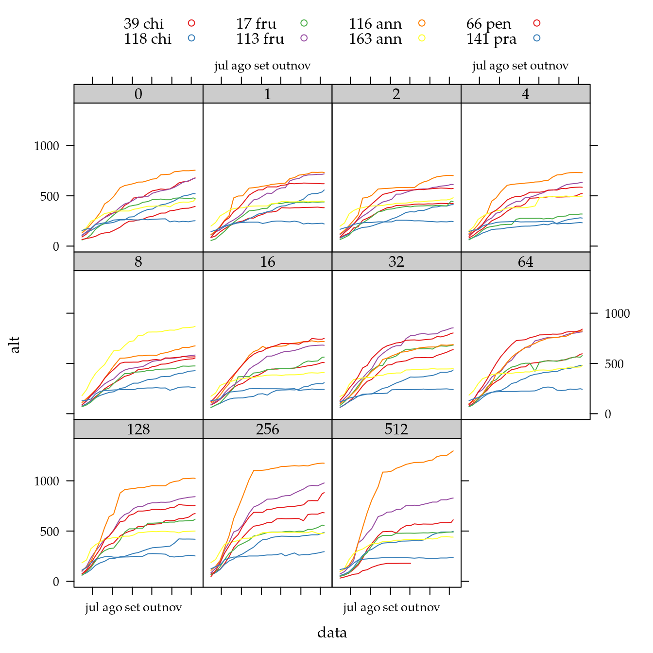
#--------------------------------------------
# Variáveis medidas nas plantas.

combineLimits(
    useOuterStrips(
        xyplot(flores + matur + nfrut + mff + msf + diamc ~
                   log2(dose + 1) | genab,
               outer = TRUE,
               scales = list(y = list(relation = "free")),
               data = cn$planta))) +
    layer(panel.smoother(x, y,
                         method = "lm",
                         form = y ~ poly(x, degree = 2), ...))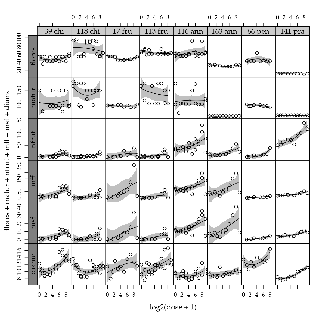
#--------------------------------------------
# Variáveis medidas nos frutos.

xyplot(diamf + compf ~ log2(dose + 1) | genab,
       as.table = TRUE,
       auto.key = list(columns = 2),
       data = cn$fruto) +
    glayer(panel.smoother(x, y,
                          method = "lm",
                          form = y ~ poly(x, degree = 2), ...))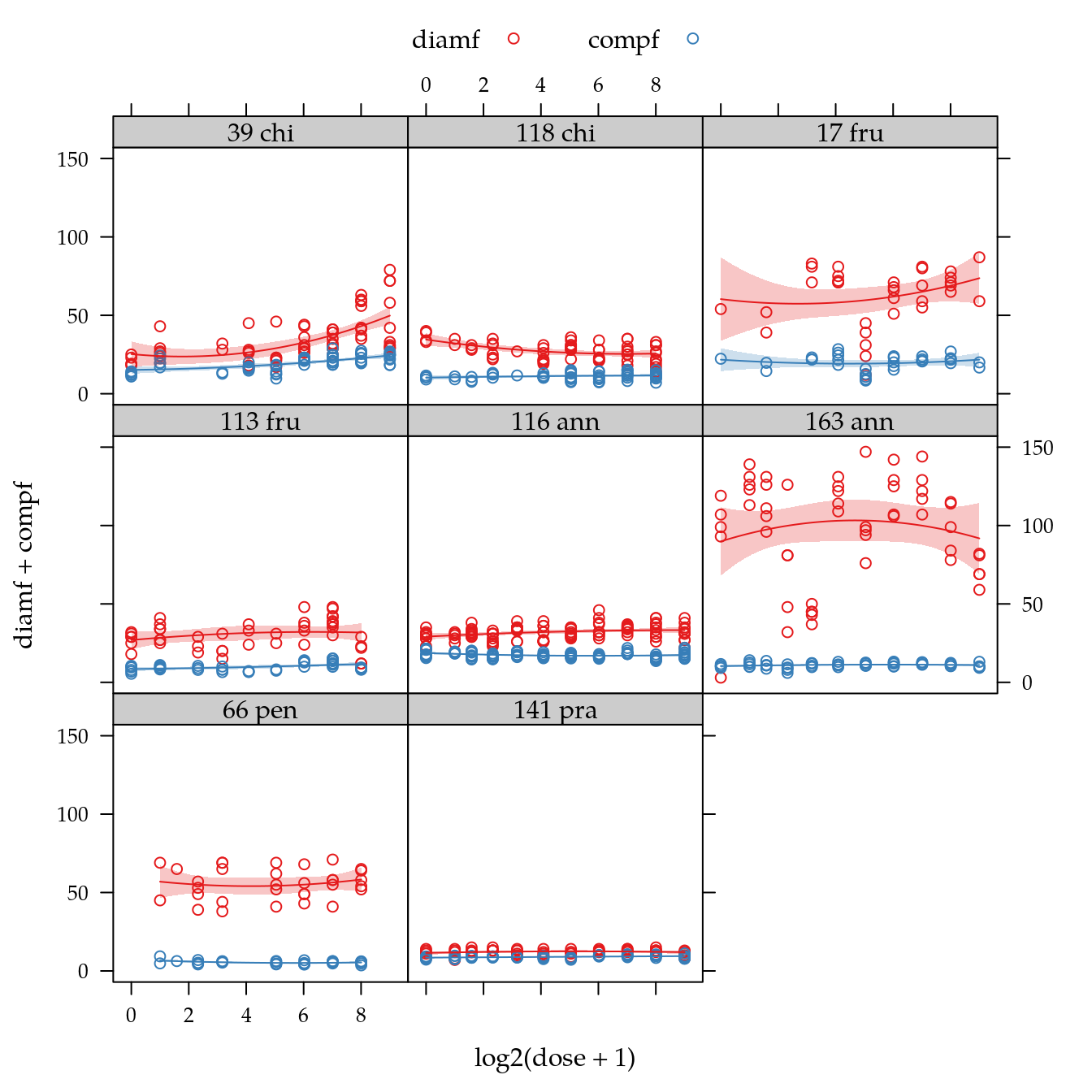
#--------------------------------------------
# Teores de substâncias determinados nos frutos.

combineLimits(
    useOuterStrips(
        xyplot(ddph + lico + bcaro + polifen + flavon + antoc ~
                   log2(dose + 1) | genab,
               outer = TRUE,
               data = cn$teor,
               scales = list(y = list(relation = "free")),
               as.table = TRUE))) +
    layer(panel.smoother(x, y,
                         method = "lm",
                         form = y ~ poly(x, degree = 2), ...))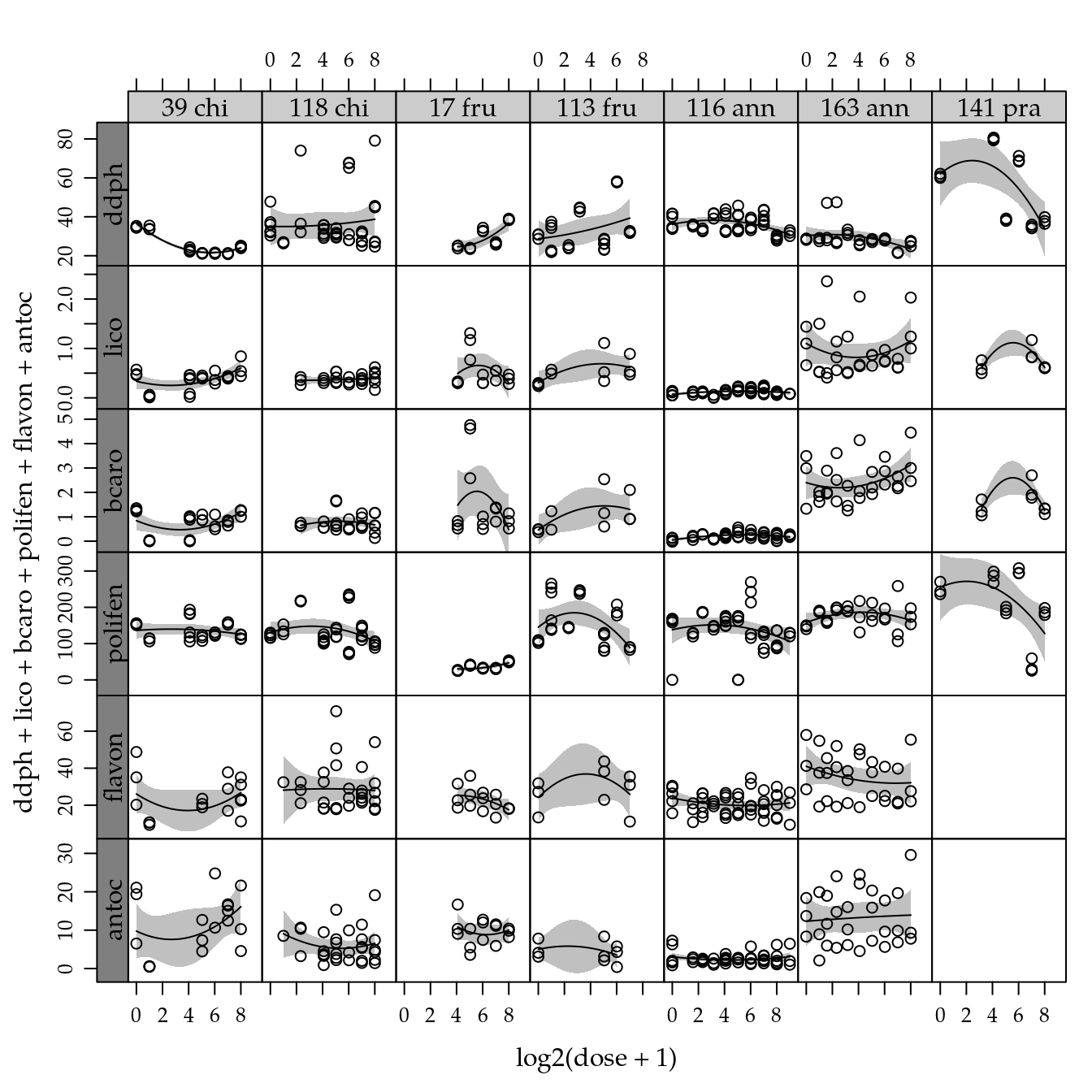
Análise do crescimento
Para simplificar, vamos trocar o problema de modelar as curvas de crescimento para fazer a análise do tamanho final das plantas. O último registro de altura de cada planta será determinado. A partir destes valores, será feita a especificação de um modelo para avaliar o efeito de genótipos e doses de nitrogênio.
# Extraí o último registro de altura por unidade experimental.
da <- ddply(.data = cn$cres,
            .variables = .(gen, dose, rept),
            .fun = function(x) {
                i <- !is.na(x$alt)
                tail(x[order(x$data), ][i, ], n = 1)
            })
da$ldose <- log2(da$dose + 1)

xtabs(~data, data = da)
## data
## 2016-10-02 2016-12-07
## 1 130# Remove observações indesejáveis.
da <- subset(da,
data == max(data) &
!(genab == "163 ann" & alt > 600))
# Verifica o efeito de nitrogênio e genótipo na altura (outliers
# removidos).
xyplot(alt ~ ldose | genab,
data = da) +
layer(panel.smoother(x, y,
method = "lm",
form = y ~ poly(x, degree = 2), ...))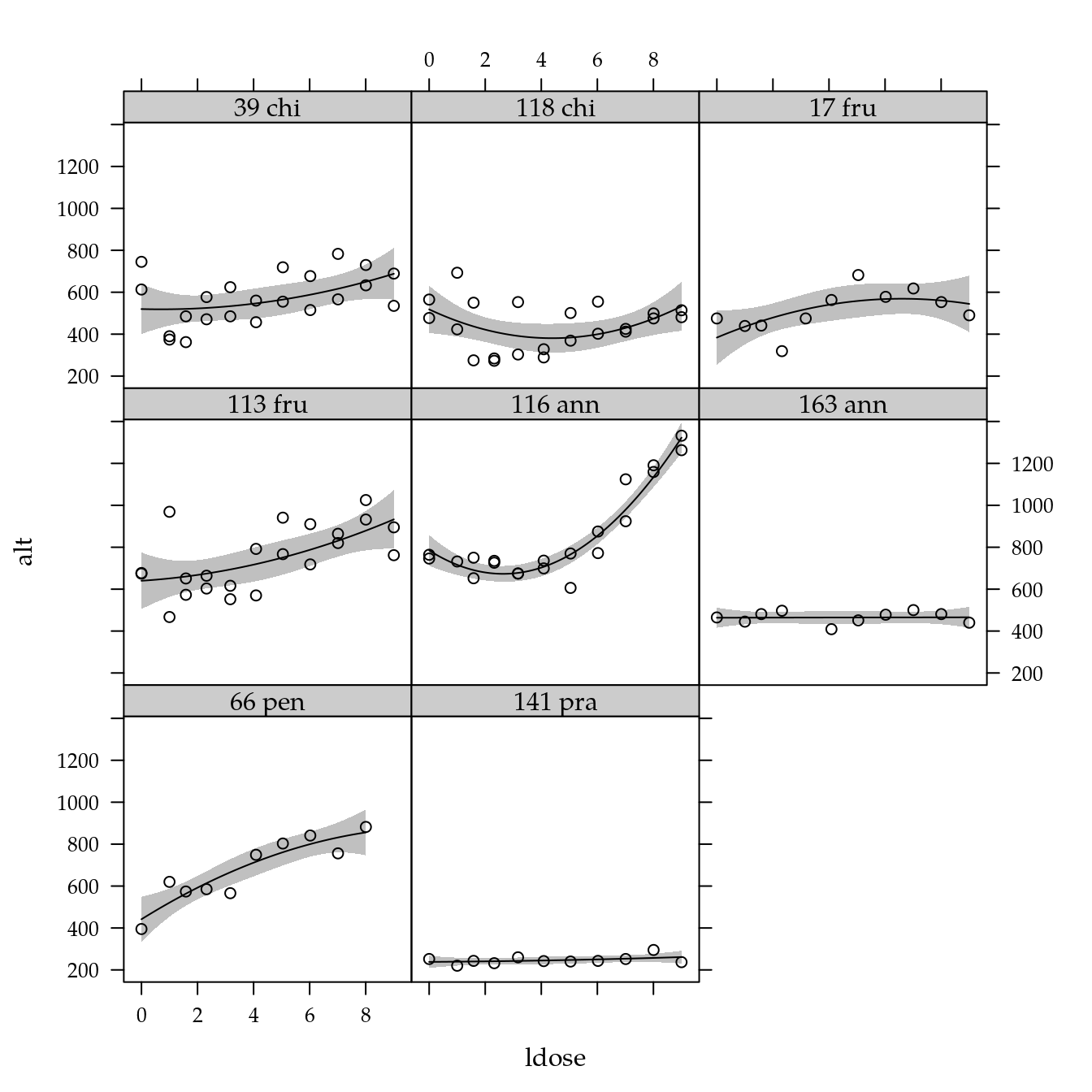
A análise exploratória dos dados, enriquecida com o ajuste de modelos separado por nível de genótipo, sugere a existência de interação entre o efeito de genótipos e nitrogênio, ou seja, para cada genótipo o efeito de nitrogênio se manifesta de forma particular. Os gráficos sugerem que um polinômio de grau 2 é suficiente para expressar o efeito de nitrogênio.
# Modelo saturado considerando dose como fator categórico.
m0 <- lm(alt ~ genab * factor(dose),
         data = da)
anova(m0)
## Analysis of Variance Table
##
## Response: alt
## Df Sum Sq Mean Sq F value Pr(>F)
## genab 7 4101154 585879 51.6411 < 2.2e-16 ***
## factor(dose) 10 827193 82719 7.2911 1.321e-06 ***
## genab:factor(dose) 68 1082505 15919 1.4032 0.118
## Residuals 43 487844 11345
## ---
## Signif. codes: 0 '***' 0.001 '**' 0.01 '*' 0.05 '.' 0.1 ' ' 1# Modelo que expressa o efeito de dose com polinômio de grau 2.
m1 <- update(m0, . ~ genab * poly(ldose, degree = 2))
anova(m1)## Analysis of Variance Table
##
## Response: alt
## Df Sum Sq Mean Sq F value Pr(>F)
## genab 7 4101154 585879 63.6764 < 2.2e-16
## poly(ldose, degree = 2) 2 700733 350367 38.0797 3.666e-13
## genab:poly(ldose, degree = 2) 14 730717 52194 5.6727 4.576e-08
## Residuals 105 966092 9201
##
## genab ***
## poly(ldose, degree = 2) ***
## genab:poly(ldose, degree = 2) ***
## Residuals
## ---
## Signif. codes: 0 '***' 0.001 '**' 0.01 '*' 0.05 '.' 0.1 ' ' 1# Verifica se o modelo reduzido difere do saturado.
anova(m1, m0)## Analysis of Variance Table
##
## Model 1: alt ~ genab + poly(ldose, degree = 2) + genab:poly(ldose, degree = 2)
## Model 2: alt ~ genab * factor(dose)
## Res.Df RSS Df Sum of Sq F Pr(>F)
## 1 105 966092
## 2 43 487844 62 478248 0.6799 0.9188
# MASS::boxcox(m1)

# Quadro de anova do modelo final.
anova(m1)
## Analysis of Variance Table
##
## Response: alt
## Df Sum Sq Mean Sq F value Pr(>F)
## genab 7 4101154 585879 63.6764 < 2.2e-16
## poly(ldose, degree = 2) 2 700733 350367 38.0797 3.666e-13
## genab:poly(ldose, degree = 2) 14 730717 52194 5.6727 4.576e-08
## Residuals 105 966092 9201
##
## genab ***
## poly(ldose, degree = 2) ***
## genab:poly(ldose, degree = 2) ***
## Residuals
## ---
## Signif. codes: 0 '***' 0.001 '**' 0.01 '*' 0.05 '.' 0.1 ' ' 1# Predição.
pred <- with(da,
expand.grid(genab = levels(genab),
ldose = seq(min(ldose),
max(ldose),
length.out = 30),
KEEP.OUT.ATTRS = FALSE))
# Obtém os valores preditos segundo o modelo ajustado.
pred <- cbind(pred,
as.data.frame(predict(m1,
newdata = pred,
interval = "confidence")))
# Legendas para os eixos.
labs <- list(
xlab = expression("Dose de nitrogênio" ~
(log[2](x + 1) * ", " * mg ~ dm^{-3})),
ylab = "Altura final das plantas (mm)")
# Gráfico dos resultados.
xyplot(alt ~ ldose | genab,
data = da,
xlab = labs$xlab,
ylab = labs$ylab) +
as.layer(
xyplot(fit + lwr + upr ~ ldose | genab,
col = c("black", "gray", "gray"),
data = pred,
type = "l"))
# Rescrevendo o modelo para mais fácil interpretar os parâmetros.
m2 <- update(m0, . ~ 0 + genab/(ldose + I(ldose^2)))
all.equal(deviance(m2), deviance(m1))
## [1] TRUE# Estimativas dos parâmetros \beta_0 + \beta_1 x + \beta_2 x^2 por
# genótipo.
summary(m2)##
## Call:
## lm(formula = alt ~ genab + genab:ldose + genab:I(ldose^2) - 1,
## data = da)
##
## Residuals:
## Min 1Q Median 3Q Max
## -184.22 -48.62 -2.89 37.02 317.78
##
## Coefficients:
## Estimate Std. Error t value Pr(>|t|)
## genab39 chi 519.754659 51.300261 10.132 < 2e-16 ***
## genab118 chi 518.286383 51.300261 10.103 < 2e-16 ***
## genab17 fru 383.705582 72.549525 5.289 6.76e-07 ***
## genab113 fru 639.976902 51.300261 12.475 < 2e-16 ***
## genab116 ann 784.829914 54.239670 14.470 < 2e-16 ***
## genab163 ann 463.632246 72.550422 6.390 4.63e-09 ***
## genab66 pen 441.636219 75.482750 5.851 5.62e-08 ***
## genab141 pra 238.201020 72.549525 3.283 0.00139 **
## genab39 chi:ldose -3.410370 27.197755 -0.125 0.90045
## genab118 chi:ldose -62.668106 27.197755 -2.304 0.02318 *
## genab17 fru:ldose 56.153203 38.463435 1.460 0.14730
## genab113 fru:ldose 8.583363 27.197755 0.316 0.75294
## genab116 ann:ldose -84.710762 27.737260 -3.054 0.00286 **
## genab163 ann:ldose 0.273485 39.687218 0.007 0.99451
## genab66 pen:ldose 83.184525 44.744312 1.859 0.06581 .
## genab141 pra:ldose 0.873973 38.463435 0.023 0.98192
## genab39 chi:I(ldose^2) 2.455981 2.911886 0.843 0.40090
## genab118 chi:I(ldose^2) 7.141452 2.911886 2.453 0.01583 *
## genab17 fru:I(ldose^2) -4.254915 4.118028 -1.033 0.30387
## genab113 fru:I(ldose^2) 2.659439 2.911886 0.913 0.36317
## genab116 ann:I(ldose^2) 16.045749 2.938317 5.461 3.20e-07 ***
## genab163 ann:I(ldose^2) -0.004893 4.299210 -0.001 0.99909
## genab66 pen:I(ldose^2) -3.926453 5.369439 -0.731 0.46625
## genab141 pra:I(ldose^2) 0.186830 4.118028 0.045 0.96390
## ---
## Signif. codes: 0 '***' 0.001 '**' 0.01 '*' 0.05 '.' 0.1 ' ' 1
##
## Residual standard error: 95.92 on 105 degrees of freedom
## Multiple R-squared: 0.9813, Adjusted R-squared: 0.977
## F-statistic: 229.5 on 24 and 105 DF, p-value: < 2.2e-16# Para abandonar termos, considerar nível de 10%.
coeffs <- as.data.frame(summary(m2)$coefficients)
subset(coeffs, `Pr(>|t|)` < 0.2, select = c(1, 4))## Estimate Pr(>|t|)
## genab39 chi 519.754659 3.103026e-17
## genab118 chi 518.286383 3.598030e-17
## genab17 fru 383.705582 6.756324e-07
## genab113 fru 639.976902 1.865773e-22
## genab116 ann 784.829914 9.402700e-27
## genab163 ann 463.632246 4.634620e-09
## genab66 pen 441.636219 5.615689e-08
## genab141 pra 238.201020 1.394209e-03
## genab118 chi:ldose -62.668106 2.318213e-02
## genab17 fru:ldose 56.153203 1.473000e-01
## genab116 ann:ldose -84.710762 2.861462e-03
## genab66 pen:ldose 83.184525 6.581189e-02
## genab118 chi:I(ldose^2) 7.141452 1.583395e-02
## genab116 ann:I(ldose^2) 16.045749 3.197429e-07# Função que cria um dummy ou indicadora o nível do fator fornecido.
d <- function(factor, level) {
as.integer(factor == level)
}
# Declarando o polinômio de grau adequado para cada nível de genótipo.
m3 <- update(m0, . ~ genab * ldose +
d(genab, "118 chi"):I(ldose^2) +
d(genab, "116 ann"):I(ldose^2))
# summary(m3)
anova(m3, m2)## Analysis of Variance Table
##
## Model 1: alt ~ genab + ldose + genab:ldose + d(genab, "118 chi"):I(ldose^2) +
## I(ldose^2):d(genab, "116 ann")
## Model 2: alt ~ genab + genab:ldose + genab:I(ldose^2) - 1
## Res.Df RSS Df Sum of Sq F Pr(>F)
## 1 111 995074
## 2 105 966092 6 28982 0.525 0.7882# Nova predição com o modelo reduzido.
pred <- cbind(pred[, 1:2],
as.data.frame(predict(m3,
newdata = pred,
interval = "confidence")))
# Gráfico dos resultados.
xyplot(alt ~ ldose | genab,
data = da,
xlab = labs$xlab,
ylab = labs$ylab) +
as.layer(
xyplot(fit + lwr + upr ~ ldose | genab,
col = c("black", "gray", "gray"),
data = pred,
type = "l"))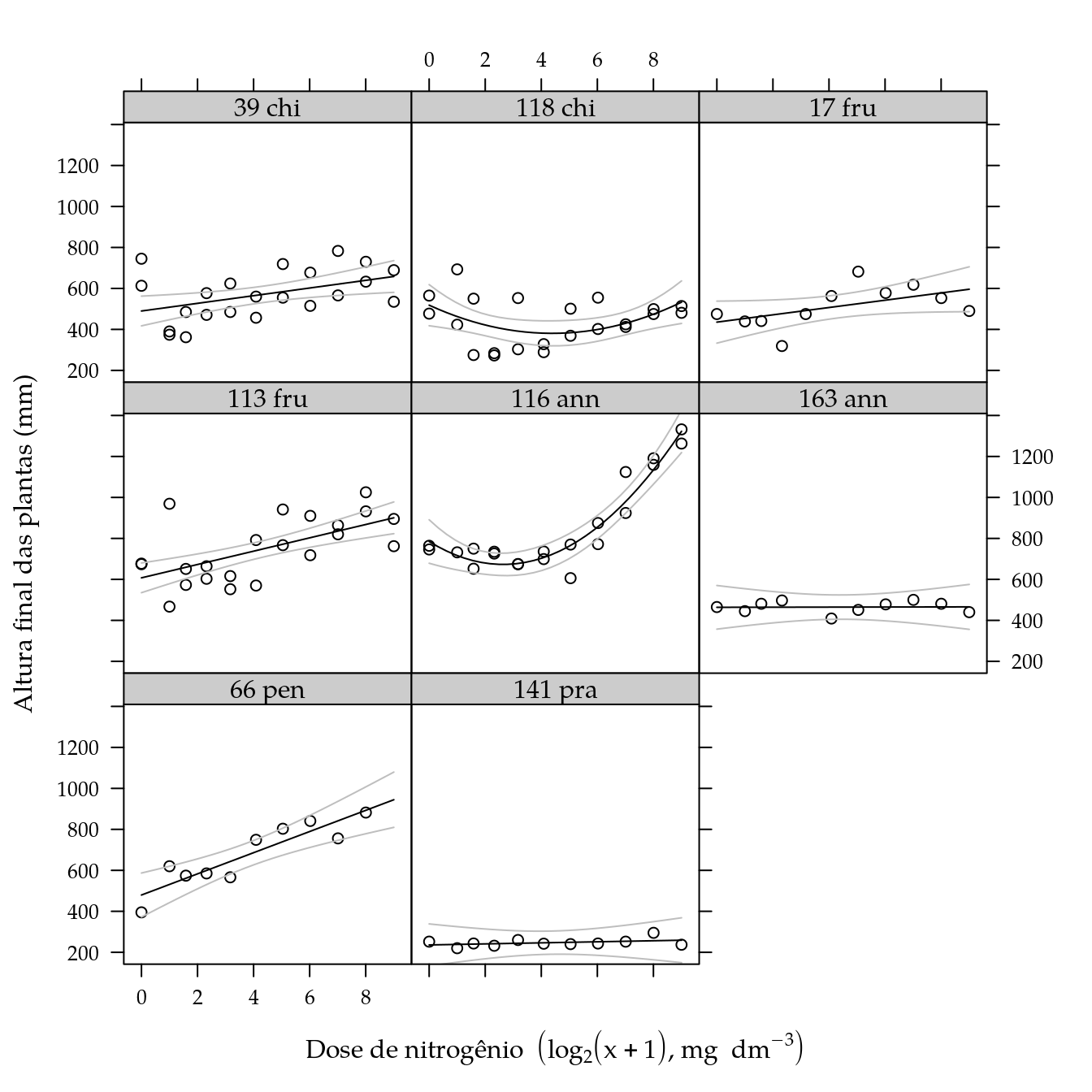
Variáveis de planta
# Estrutura dos dados de planta.
str(cn$planta)
## 'data.frame': 130 obs. of 10 variables:
## $ gen : Factor w/ 8 levels "39 C. chinense",..: 1 1 1 1 1 1 1 1 1 1 ...
## $ dose : int 0 1 2 4 8 16 32 64 128 256 ...
## $ rept : int 1 1 1 1 1 1 1 1 1 1 ...
## $ flores: int 53 35 53 44 53 42 53 53 53 42 ...
## $ matur : int 149 73 NA NA NA 93 95 86 95 149 ...
## $ nfrut : int 8 2 NA NA NA 1 1 29 13 13 ...
## $ mff : num 8.47 8.36 NA NA NA ...
## $ msf : num 0.98 0.95 NA NA NA ...
## $ diamc : num 12.33 9.46 8.89 9.3 9.03 ...
## $ genab : Factor w/ 8 levels "39 chi","118 chi",..: 1 1 1 1 1 1 1 1 1 1 ...# Frequência dos dados.
xtabs(~genab + dose, data = cn$planta)## dose
## genab 0 1 2 4 8 16 32 64 128 256 512
## 39 chi 2 2 2 2 2 2 2 2 2 2 2
## 118 chi 2 2 2 2 2 2 2 2 2 2 2
## 17 fru 1 1 1 1 1 1 1 1 1 1 1
## 113 fru 2 2 2 2 2 2 2 2 2 2 2
## 116 ann 2 1 2 2 2 2 2 2 2 2 2
## 163 ann 1 1 1 1 1 1 1 1 1 1 1
## 66 pen 1 1 1 1 1 1 1 1 1 1 0
## 141 pra 1 1 1 1 1 1 1 1 1 1 1# A dose transformada será usada em todas as análises.
cn$planta$ldose <- log2(cn$planta$dose + 1)Florescimento
# Exploratória.
xyplot(flores ~ ldose | genab,
       data = cn$planta) +
    layer(panel.smoother(x, y,
                         method = "lm",
                         form = y ~ poly(x, degree = 2), ...))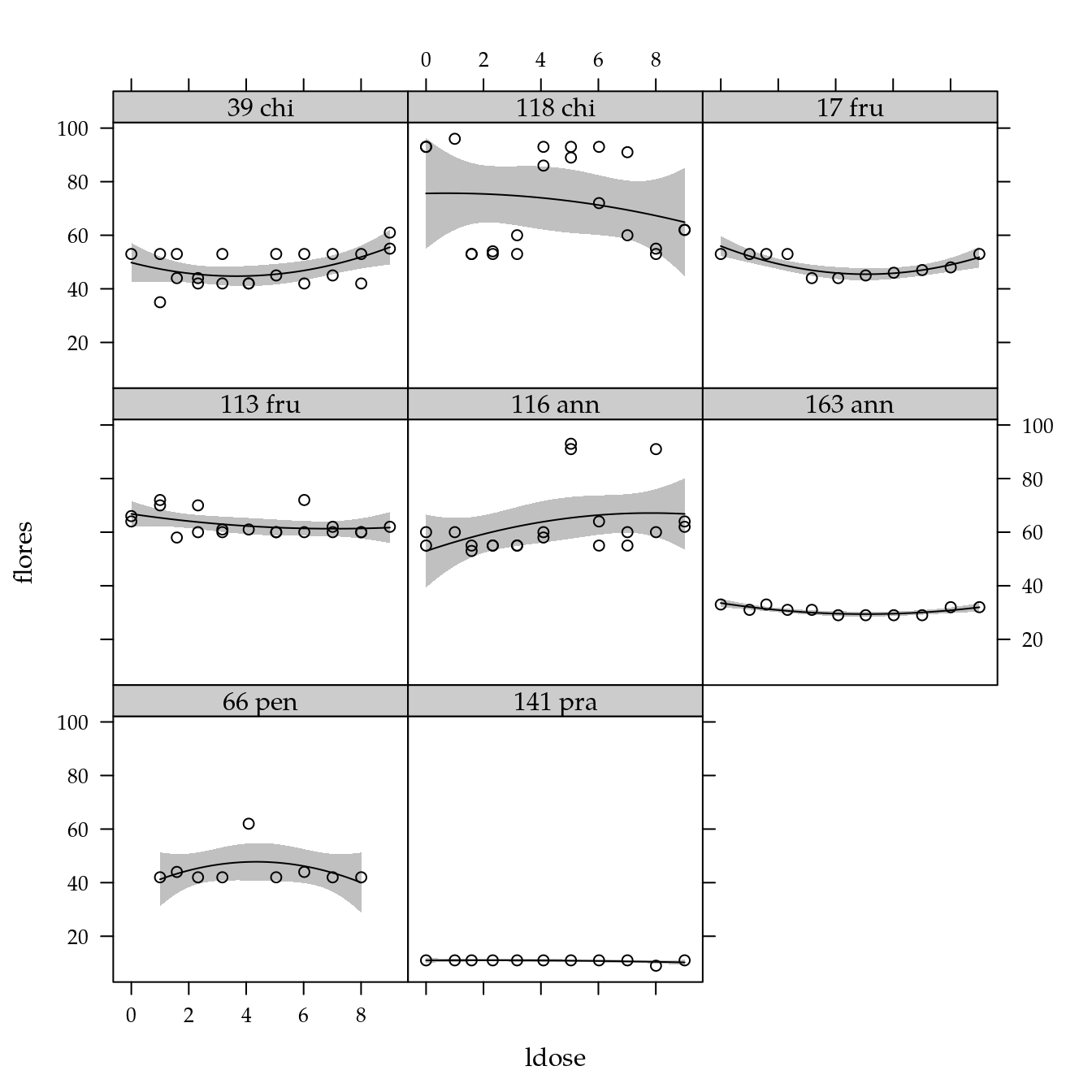
# Declara modelo fatorial com dose expresso por polinômio de grau 2.
m0 <- lm(flores ~ genab * poly(ldose, degree = 2),
         data = cn$planta)
anova(m0)
## Analysis of Variance Table
##
## Response: flores
## Df Sum Sq Mean Sq F value Pr(>F)
## genab 7 37844 5406.3 52.7103 <2e-16 ***
## poly(ldose, degree = 2) 2 16 8.1 0.0787 0.9244
## genab:poly(ldose, degree = 2) 14 1172 83.7 0.8165 0.6497
## Residuals 100 10257 102.6
## ---
## Signif. codes: 0 '***' 0.001 '**' 0.01 '*' 0.05 '.' 0.1 ' ' 1# par(mfrow = c(2, 2))
# plot(m0); layout(1)
# MASS::boxcox(m0)
# Declara o modelo reduzido contendo apenas o efeito de genótipo.
m1 <- update(m0, . ~ genab)
anova(m1, m0)## Analysis of Variance Table
##
## Model 1: flores ~ genab
## Model 2: flores ~ genab * poly(ldose, degree = 2)
## Res.Df RSS Df Sum of Sq F Pr(>F)
## 1 116 11445
## 2 100 10257 16 1188.6 0.7243 0.7634# Comparações múltiplas entre médias de genótipos.
L <- LE_matrix(m1, effect = "genab")
rownames(L) <- attr(L, "grid")$genab
pred <- apmc(L, m1, "genab", test = "fdr")
arrange(pred, -fit)## genab fit lwr upr cld
## 1 118 chi 72.23810 67.944938 76.53125 a
## 2 113 fru 63.05263 58.539171 67.56609 b
## 3 116 ann 62.66667 58.373509 66.95982 b
## 4 17 fru 49.00000 43.068151 54.93185 c
## 5 39 chi 47.85714 43.563985 52.15030 c
## 6 66 pen 44.66667 38.108760 51.22457 c
## 7 163 ann 30.81818 24.886332 36.75003 d
## 8 141 pra 10.81818 4.886332 16.75003 e# Gráfico de segmentos.
segplot(reorder(genab, fit) ~ lwr + upr,
centers = fit,
data = pred,
cld = sprintf("%0.1f %s", pred$fit, pred$cld),
draw = FALSE,
xlab = "Dias para o florescimento",
ylab = "Genótipo de pimenta") +
layer(panel.text(x = centers,
y = z,
labels = cld,
pos = 3))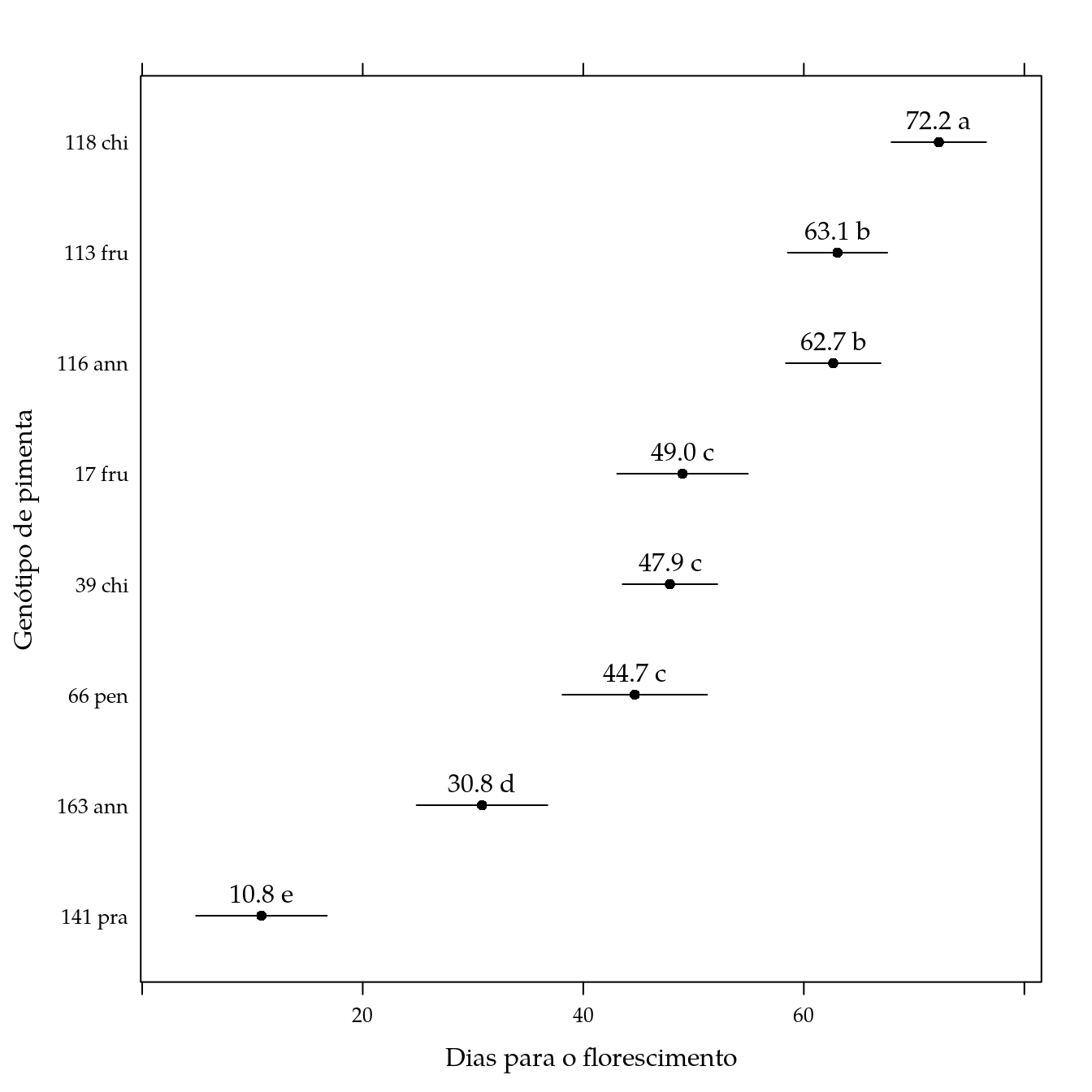
Maturação
# Exploratória.
xyplot(matur ~ ldose | genab,
       data = cn$planta) +
    layer(panel.smoother(x, y,
                         method = "lm",
                         form = y ~ poly(x, degree = 2), ...))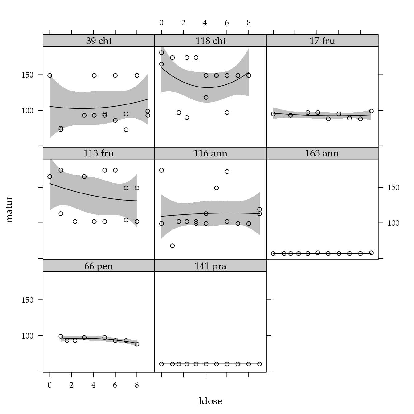
# Declara modelo fatorial com dose expresso por polinômio de grau 2.
m0 <- lm(matur ~ genab * poly(ldose, degree = 2),
         data = cn$planta)
anova(m0)
## Analysis of Variance Table
##
## Response: matur
## Df Sum Sq Mean Sq F value Pr(>F)
## genab 7 94121 13445.8 21.2499 2.786e-16
## poly(ldose, degree = 2) 2 666 333.2 0.5266 0.5925
## genab:poly(ldose, degree = 2) 14 2253 160.9 0.2543 0.9969
## Residuals 85 53784 632.7
##
## genab ***
## poly(ldose, degree = 2)
## genab:poly(ldose, degree = 2)
## Residuals
## ---
## Signif. codes: 0 '***' 0.001 '**' 0.01 '*' 0.05 '.' 0.1 ' ' 1# par(mfrow = c(2, 2))
# plot(m0); layout(1)
# MASS::boxcox(m0)
# Declara o modelo reduzido contendo apenas o efeito de genótipo.
m1 <- update(m0, . ~ genab)
anova(m1, m0)## Analysis of Variance Table
##
## Model 1: matur ~ genab
## Model 2: matur ~ genab * poly(ldose, degree = 2)
## Res.Df RSS Df Sum of Sq F Pr(>F)
## 1 101 56703
## 2 85 53784 16 2919.2 0.2883 0.9964# Comparações múltiplas entre médias de genótipos.
L <- LE_matrix(m1, effect = "genab")
rownames(L) <- attr(L, "grid")$genab
pred <- apmc(L, m1, "genab", test = "fdr")
arrange(pred, -fit)## genab fit lwr upr cld
## 1 118 chi 142.16667 131.08799 153.24534 a
## 2 113 fru 140.33333 128.19725 152.46942 a
## 3 116 ann 112.47619 102.21933 122.73305 b
## 4 39 chi 107.06250 95.31179 118.81321 b
## 5 66 pen 94.12500 77.50699 110.74301 b
## 6 17 fru 93.44444 77.77683 109.11206 b
## 7 141 pra 60.00000 45.82811 74.17189 c
## 8 163 ann 57.18182 43.00993 71.35371 c# Gráfico de segmentos.
segplot(reorder(genab, fit) ~ lwr + upr,
centers = fit,
data = pred,
cld = sprintf("%0.1f %s", pred$fit, pred$cld),
draw = FALSE,
xlab = "Dias para a maturação dos frutos",
ylab = "Genótipo de pimenta") +
layer(panel.text(x = centers,
y = z,
labels = cld,
pos = 3))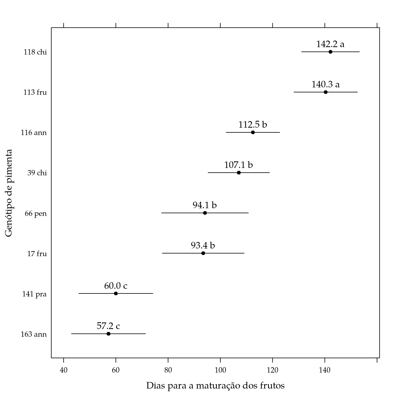
Número de frutos
# Exploratória.
xyplot(nfrut ~ ldose | genab,
       data = cn$planta) +
    layer(panel.smoother(x, y,
                         method = "lm",
                         form = y ~ poly(x, degree = 2), ...))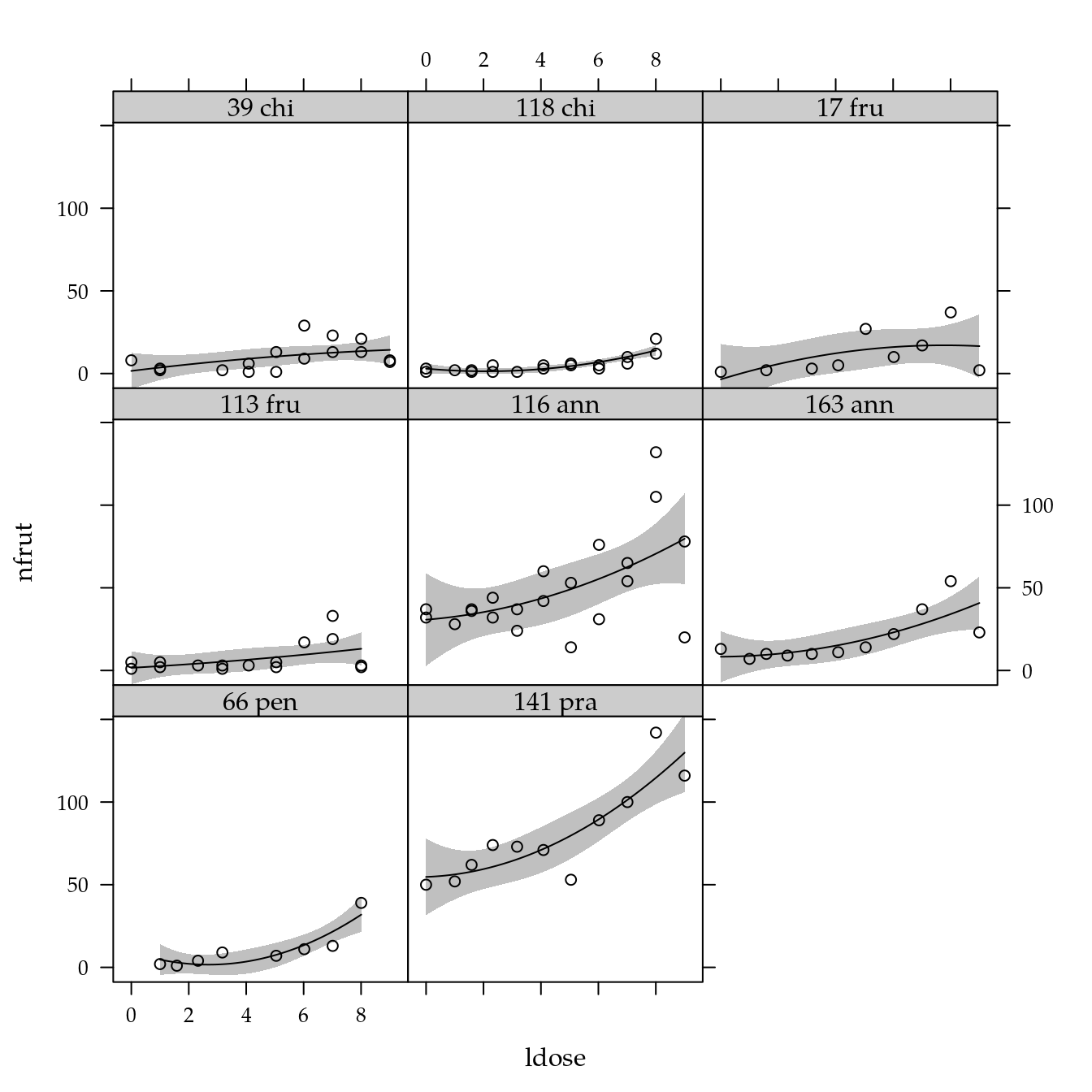
# Declara modelo fatorial com dose expresso por polinômio de grau 2.
m0 <- glm(nfrut ~ genab * poly(ldose, degree = 2),
          data = cn$planta,
          family = quasipoisson)
anova(m0, test = "F")
## Analysis of Deviance Table
##
## Model: quasipoisson, link: log
##
## Response: nfrut
##
## Terms added sequentially (first to last)
##
##
## Df Deviance Resid. Df Resid. Dev
## NULL 108 3261.0
## genab 7 2297.42 101 963.6
## poly(ldose, degree = 2) 2 377.26 99 586.3
## genab:poly(ldose, degree = 2) 14 105.44 85 480.9
## F Pr(>F)
## NULL
## genab 58.8438 < 2.2e-16 ***
## poly(ldose, degree = 2) 33.8195 1.565e-11 ***
## genab:poly(ldose, degree = 2) 1.3503 0.1962
## ---
## Signif. codes: 0 '***' 0.001 '**' 0.01 '*' 0.05 '.' 0.1 ' ' 1# par(mfrow = c(2, 2))
# plot(m0); layout(1)
# MASS::boxcox(m0)
# Declara o modelo reduzido contendo apenas o efeito de genótipo.
m1 <- update(m0, . ~ genab + ldose)
anova(m1, m0, test = "F")## Analysis of Deviance Table
##
## Model 1: nfrut ~ genab + ldose
## Model 2: nfrut ~ genab * poly(ldose, degree = 2)
## Resid. Df Resid. Dev Df Deviance F Pr(>F)
## 1 100 586.34
## 2 85 480.89 15 105.44 1.2603 0.2455# Comparações múltiplas entre médias de genótipos.
L <- LE_matrix(m1, effect = "genab", at = list(ldose = 1))
rownames(L) <- attr(L, "grid")$genab
pred <- apmc(L, m1, "genab", test = "fdr")
# Passa a inversa da função de ligação.
pred[, c("fit", "lwr", "upr")] <-
m0$family$linkinv(pred[, c("fit", "lwr", "upr")])
arrange(pred, -fit)## genab fit lwr upr cld
## 1 141 pra 47.484809 38.184575 59.050207 a
## 2 116 ann 28.687044 23.206629 35.461699 b
## 3 163 ann 11.305907 7.894791 16.190870 c
## 4 66 pen 6.512810 3.836229 11.056872 cd
## 5 17 fru 6.350335 3.878297 10.398057 cd
## 6 39 chi 5.235121 3.459423 7.922271 d
## 7 113 fru 4.274108 2.633706 6.936236 d
## 8 118 chi 3.188195 1.911967 5.316298 d# Gráfico de segmentos.
segplot(reorder(genab, fit) ~ lwr + upr,
centers = fit,
data = pred,
cld = sprintf("%0.1f %s", pred$fit, pred$cld),
draw = FALSE,
xlab = "Número de frutos",
ylab = "Genótipo de pimenta") +
layer(panel.text(x = centers,
y = z,
labels = cld,
pos = 3))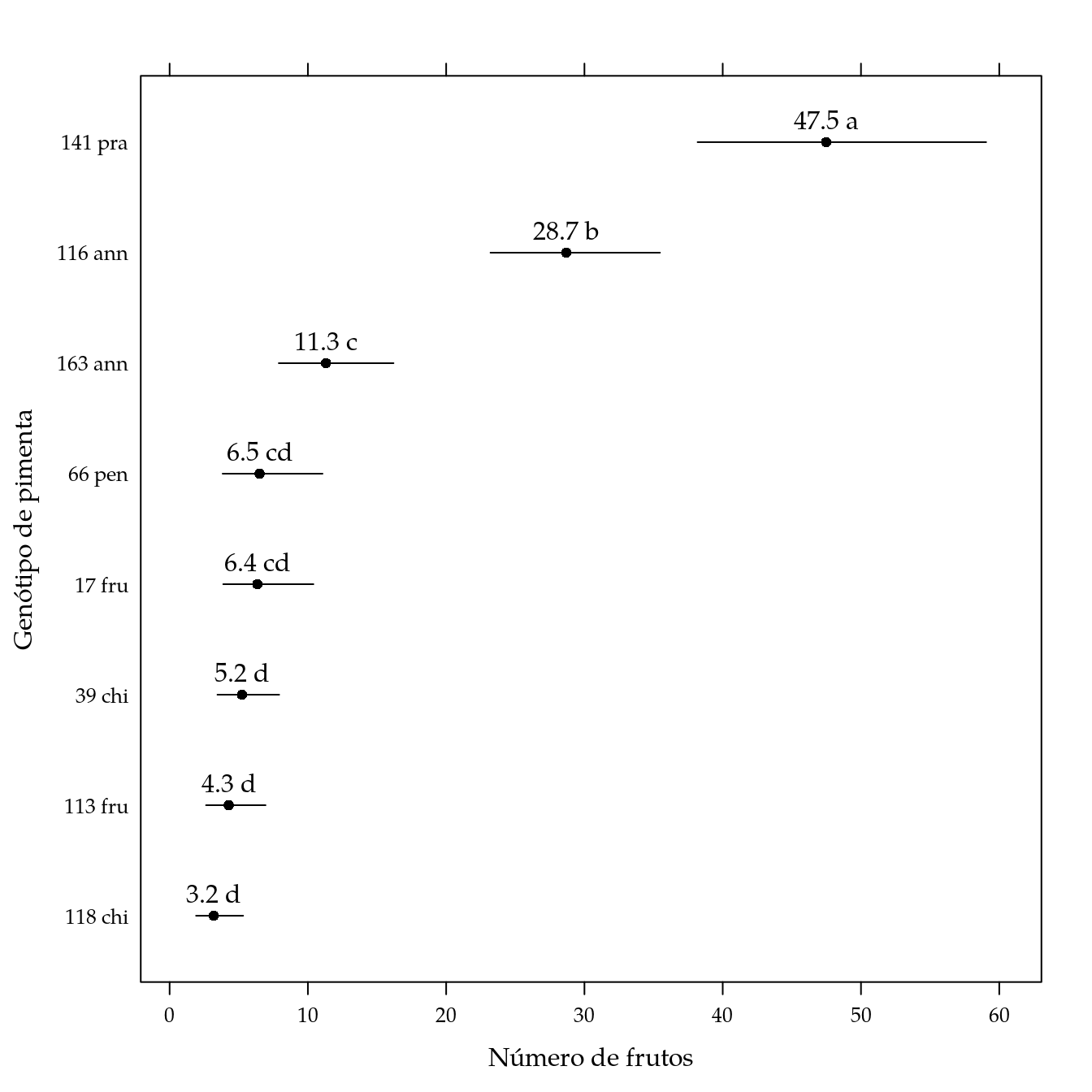
# Predição.
pred <- with(da,
             expand.grid(genab = levels(genab),
                         ldose = seq(min(ldose),
                                     max(ldose),
                                     length.out = 30),
                         KEEP.OUT.ATTRS = FALSE))
el <- predict(m1, newdata = pred, se.fit = TRUE)
me <- with(el, outer(se.fit,
                     c(fit = 0, lwr = -1, upr = 1) *
                     qt(0.975, df = df.residual(m1)),
                     FUN = "*"))
ci <- sweep(me, MARGIN = 1, STATS = el$fit, FUN = "+")
ci <- m0$family$linkinv(ci)
pred <- cbind(pred, as.data.frame(ci))

# Gráfico dos resultados.
xyplot(nfrut ~ ldose | genab,
       data = cn$planta,
       xlab = labs$xlab,
       ylab = "Número de frutos") +
    as.layer(
        xyplot(fit + lwr + upr ~ ldose | genab,
               col = c("black", "gray", "gray"),
               data = pred,
               type = "l"))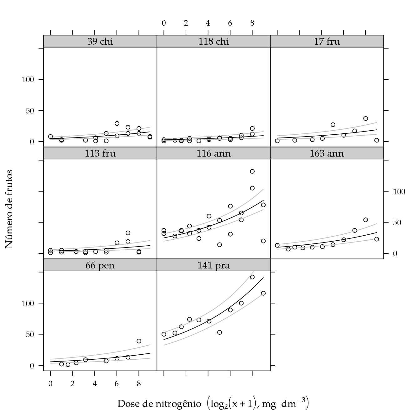
Massa fresca de frutos
# Exploratória.
xyplot(log10(mff) ~ ldose | genab,
       data = cn$planta) +
    layer(panel.smoother(x, y,
                         method = "lm",
                         form = y ~ poly(x, degree = 2), ...))
# Declara modelo fatorial com dose expresso por polinômio de grau 2.
m0 <- lm(log10(mff) ~ genab * poly(ldose, degree = 2),
         data = cn$planta)
anova(m0)
## Analysis of Variance Table
##
## Response: log10(mff)
## Df Sum Sq Mean Sq F value Pr(>F)
## genab 7 23.4846 3.3549 25.4113 < 2.2e-16
## poly(ldose, degree = 2) 2 6.7320 3.3660 25.4950 4.006e-09
## genab:poly(ldose, degree = 2) 14 2.2376 0.1598 1.2106 0.2867
## Residuals 73 9.6379 0.1320
##
## genab ***
## poly(ldose, degree = 2) ***
## genab:poly(ldose, degree = 2)
## Residuals
## ---
## Signif. codes: 0 '***' 0.001 '**' 0.01 '*' 0.05 '.' 0.1 ' ' 1# par(mfrow = c(2, 2))
# plot(m0); layout(1)
# MASS::boxcox(m0)
# Declara o modelo reduzido contendo apenas o efeito de genótipo.
m1 <- update(m0, . ~ genab + ldose)
anova(m1, m0)## Analysis of Variance Table
##
## Model 1: log10(mff) ~ genab + ldose
## Model 2: log10(mff) ~ genab * poly(ldose, degree = 2)
## Res.Df RSS Df Sum of Sq F Pr(>F)
## 1 88 12.0033
## 2 73 9.6379 15 2.3654 1.1944 0.2957# Comparações múltiplas entre médias de genótipos.
L <- LE_matrix(m1, effect = "genab", at = list(ldose = 1))
rownames(L) <- attr(L, "grid")$genab
pred <- apmc(L, m1, "genab", test = "fdr")
arrange(pred, -fit)## genab fit lwr upr cld
## 1 116 ann 1.5686837 1.3817509463 1.7556165 a
## 2 163 ann 1.4236764 1.1857412174 1.6616116 ab
## 3 17 fru 1.1521387 0.8867108912 1.4175665 bc
## 4 141 pra 1.1062212 0.8682860458 1.3441564 bc
## 5 39 chi 0.9976031 0.7764833852 1.2187228 c
## 6 113 fru 0.3437844 0.1177411183 0.5698276 d
## 7 118 chi 0.3361437 0.0943372483 0.5779502 d
## 8 66 pen 0.2740468 0.0004413492 0.5476523 d# Gráfico de segmentos.
segplot(reorder(genab, fit) ~ lwr + upr,
centers = fit,
data = pred,
cld = sprintf("%0.2f %s", pred$fit, pred$cld),
draw = FALSE,
xlab = "Massa fresca de frutos (g) (log 10)",
ylab = "Genótipo de pimenta") +
layer(panel.text(x = centers,
y = z,
labels = cld,
pos = 3))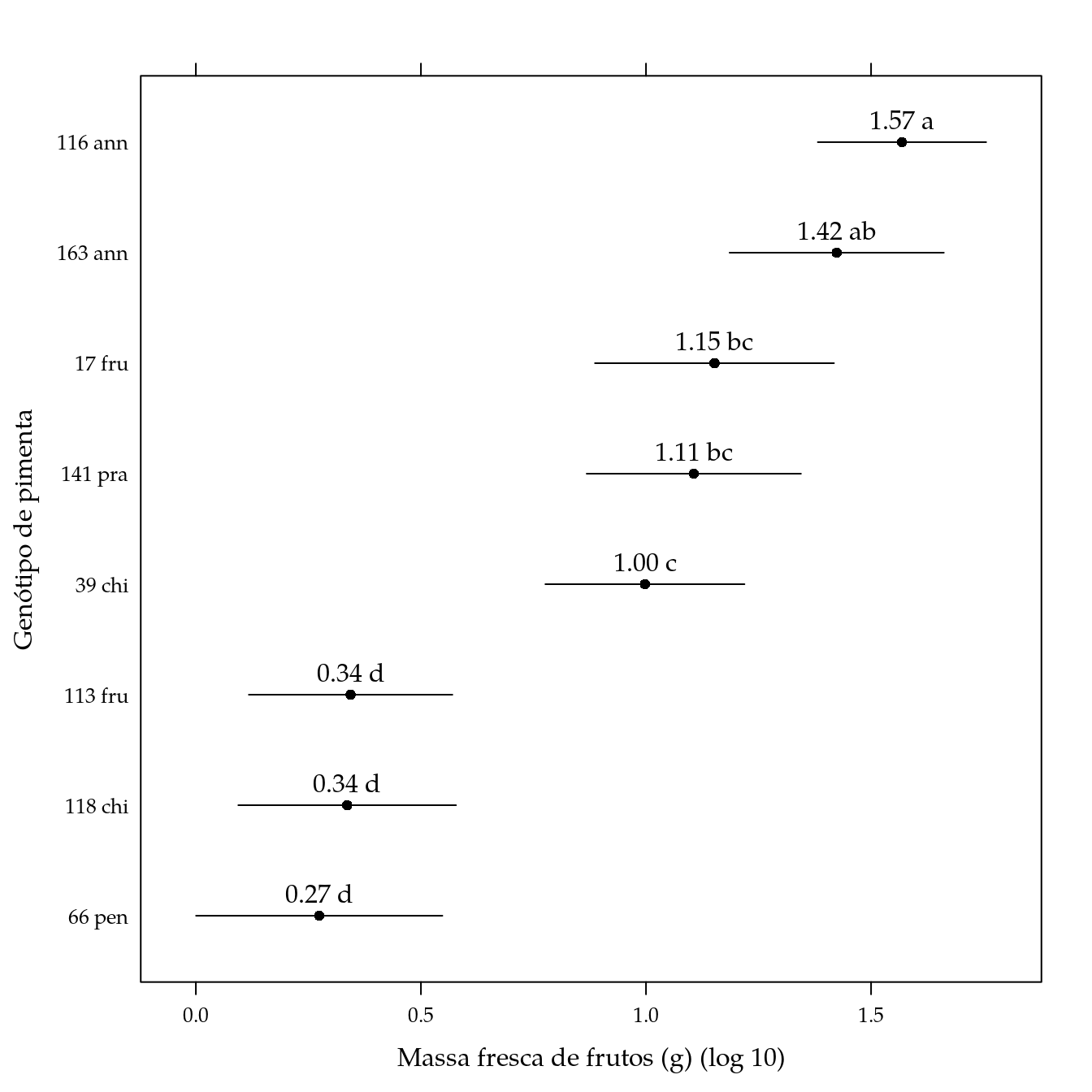
Massa seca de frutos
# Exploratória.
xyplot(log10(msf) ~ ldose | genab,
       data = cn$planta) +
    layer(panel.smoother(x, y,
                         method = "lm",
                         form = y ~ poly(x, degree = 2), ...))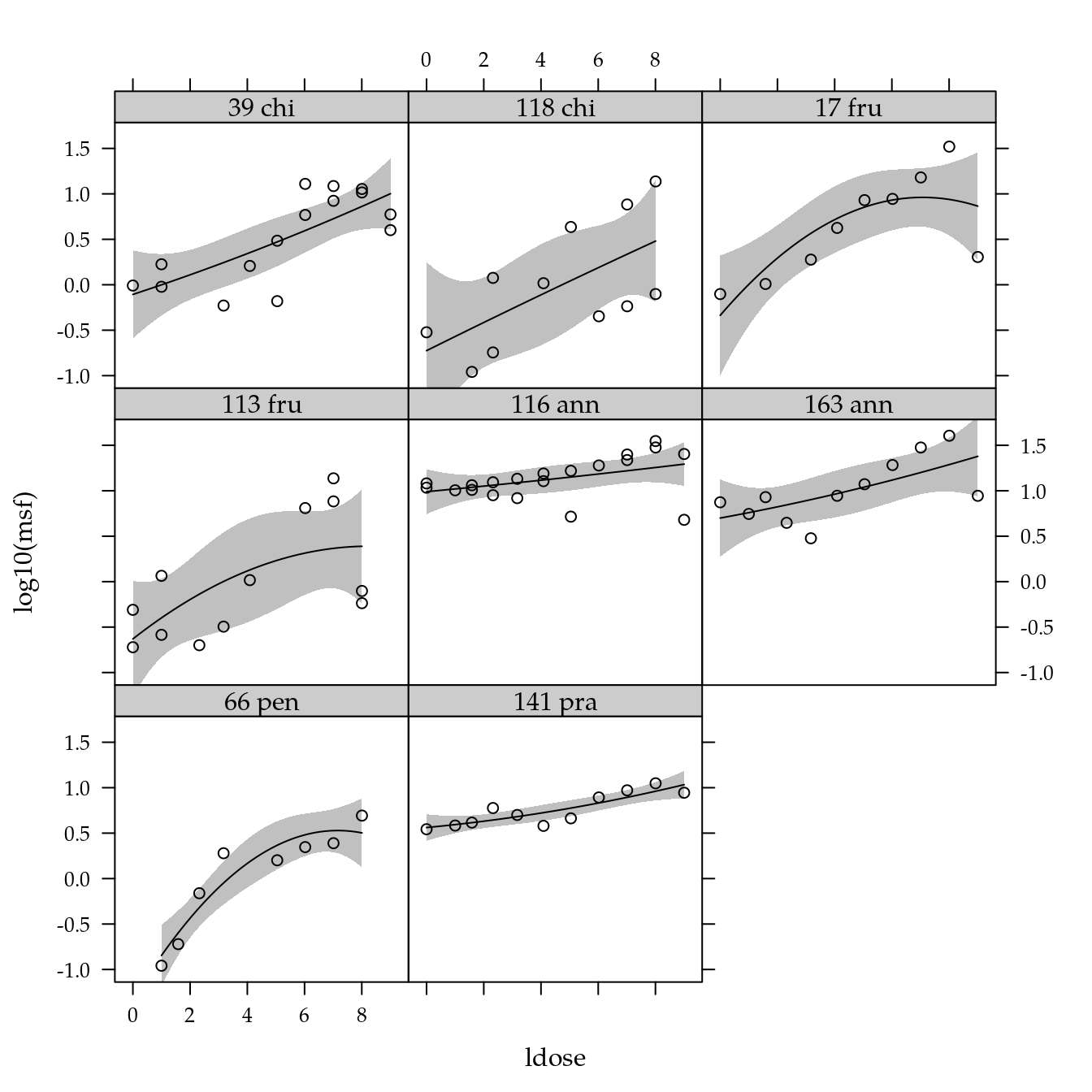
# Declara modelo fatorial com dose expresso por polinômio de grau 2.
m0 <- lm(log10(msf) ~ genab * poly(ldose, degree = 2),
         data = cn$planta)
anova(m0)
## Analysis of Variance Table
##
## Response: log10(msf)
## Df Sum Sq Mean Sq F value Pr(>F)
## genab 7 19.2620 2.7517 21.1253 2.906e-15
## poly(ldose, degree = 2) 2 7.6516 3.8258 29.3713 4.378e-10
## genab:poly(ldose, degree = 2) 14 2.3230 0.1659 1.2739 0.2446
## Residuals 73 9.5087 0.1303
##
## genab ***
## poly(ldose, degree = 2) ***
## genab:poly(ldose, degree = 2)
## Residuals
## ---
## Signif. codes: 0 '***' 0.001 '**' 0.01 '*' 0.05 '.' 0.1 ' ' 1# par(mfrow = c(2, 2))
# plot(m0); layout(1)
# MASS::boxcox(m0)
# Declara o modelo reduzido contendo apenas o efeito de genótipo.
m1 <- update(m0, . ~ genab + ldose)
anova(m1, m0)## Analysis of Variance Table
##
## Model 1: log10(msf) ~ genab + ldose
## Model 2: log10(msf) ~ genab * poly(ldose, degree = 2)
## Res.Df RSS Df Sum of Sq F Pr(>F)
## 1 88 11.9851
## 2 73 9.5087 15 2.4763 1.2674 0.245# Comparações múltiplas entre médias de genótipos.
L <- LE_matrix(m1, effect = "genab", at = list(ldose = 1))
rownames(L) <- attr(L, "grid")$genab
pred <- apmc(L, m1, "genab", test = "fdr")
arrange(pred, -fit)## genab fit lwr upr cld
## 1 116 ann 0.79807605 0.61128505 0.98486706 a
## 2 163 ann 0.67374734 0.43599261 0.91150208 ab
## 3 141 pra 0.42989615 0.19214141 0.66765089 bc
## 4 17 fru 0.24802745 -0.01719909 0.51325398 cd
## 5 39 chi 0.09532626 -0.12562575 0.31627827 d
## 6 113 fru -0.31371265 -0.53958449 -0.08784081 e
## 7 66 pen -0.31517440 -0.58857240 -0.04177639 e
## 8 118 chi -0.37852902 -0.62015215 -0.13690589 e# Gráfico de segmentos.
segplot(reorder(genab, fit) ~ lwr + upr,
centers = fit,
data = pred,
cld = sprintf("%0.2f %s", pred$fit, pred$cld),
draw = FALSE,
xlab = "Massa seca de frutos (g) (log 10)",
ylab = "Genótipo de pimenta") +
layer(panel.text(x = centers,
y = z,
labels = cld,
pos = 3))
Diametro à altura do colo
# Exploratória.
xyplot(diamc ~ ldose | genab,
       data = cn$planta) +
    layer(panel.smoother(x, y,
                         method = "lm",
                         form = y ~ poly(x, degree = 2), ...))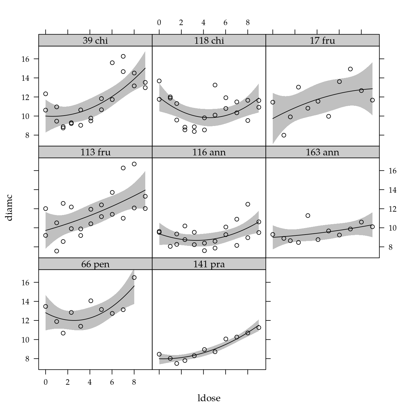
# Declara modelo fatorial com dose expresso por polinômio de grau 2.
m0 <- lm(diamc ~ genab * poly(ldose, degree = 2),
         data = cn$planta)
anova(m0)
## Analysis of Variance Table
##
## Response: diamc
## Df Sum Sq Mean Sq F value Pr(>F)
## genab 7 179.687 25.670 12.5335 1.282e-11
## poly(ldose, degree = 2) 2 107.453 53.726 26.2327 5.555e-10
## genab:poly(ldose, degree = 2) 14 52.947 3.782 1.8466 0.04093
## Residuals 106 217.095 2.048
##
## genab ***
## poly(ldose, degree = 2) ***
## genab:poly(ldose, degree = 2) *
## Residuals
## ---
## Signif. codes: 0 '***' 0.001 '**' 0.01 '*' 0.05 '.' 0.1 ' ' 1# par(mfrow = c(2, 2))
# plot(m0); layout(1)
# MASS::boxcox(m0)
# Declara o modelo reduzido contendo apenas o efeito de genótipo.
m1 <- update(m0, . ~ genab * ldose)
anova(m1, m0)## Analysis of Variance Table
##
## Model 1: diamc ~ genab + ldose + genab:ldose
## Model 2: diamc ~ genab * poly(ldose, degree = 2)
## Res.Df RSS Df Sum of Sq F Pr(>F)
## 1 114 245.31
## 2 106 217.09 8 28.21 1.7217 0.1016# Predição.
pred <- with(da,
expand.grid(genab = levels(genab),
ldose = seq(min(ldose),
max(ldose),
length.out = 30),
KEEP.OUT.ATTRS = FALSE))
ci <- predict(m1, newdata = pred, interval = "confidence")
pred <- cbind(pred, as.data.frame(ci))
# Gráfico dos resultados.
xyplot(diamc ~ ldose | genab,
data = cn$planta,
xlab = labs$xlab,
ylab = "Diâmetro à altura do colo (mm)") +
as.layer(
xyplot(fit + lwr + upr ~ ldose | genab,
col = c("black", "gray", "gray"),
data = pred,
type = "l"))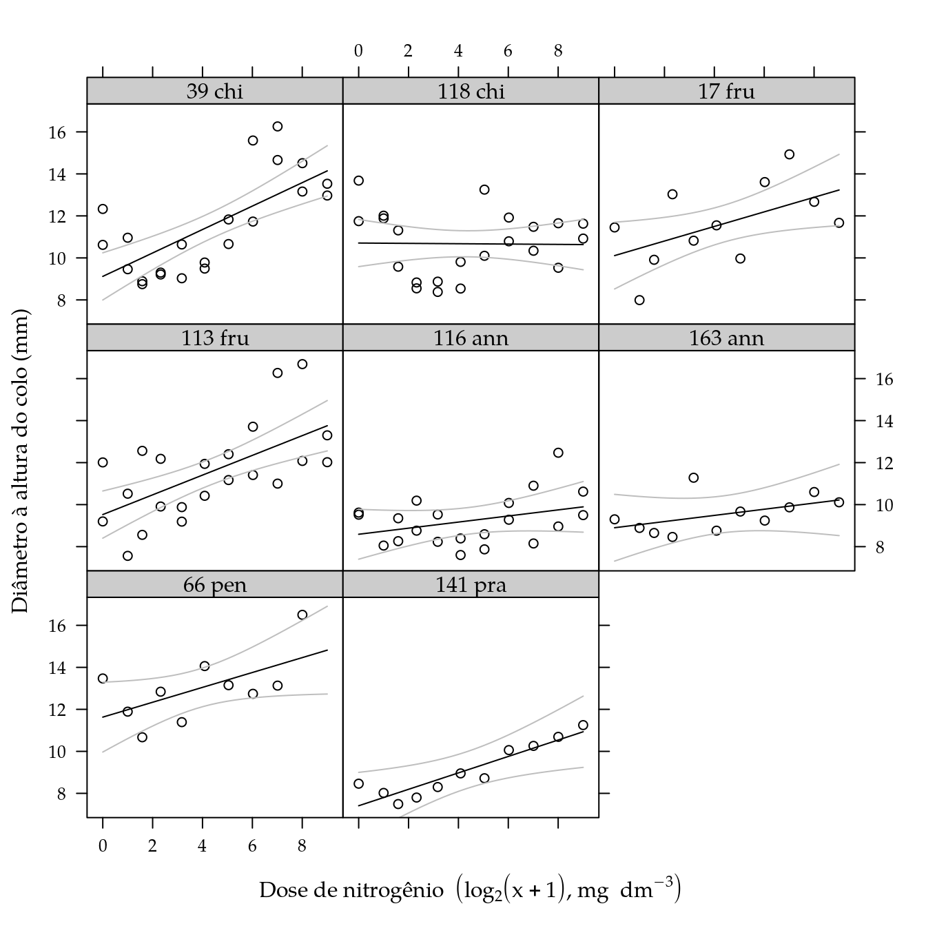
Análise canônica discriminante
#-----------------------------------------------------------------------
# Análise multivariada.

# Verificar o tamanho da tabela caso completo.
db <- cn$planta[complete.cases(cn$planta), ]
nrow(db)/nrow(cn$planta)
## [1] 0.7461538# Frequência dos dados completos.
addmargins(xtabs(~gen + dose, data = db))## dose
## gen 0 1 2 4 8 16 32 64 128 256 512
## 39 C. chinense 1 2 0 0 1 1 2 2 2 2 2
## 118 C. chinense 1 0 1 2 0 1 1 1 2 2 0
## 17 C. frutescens 1 0 1 0 1 1 1 1 1 1 1
## 113 C. frutescens 2 2 0 1 1 1 0 1 2 2 0
## 116 C. annuun 2 1 2 2 2 2 2 1 2 2 2
## 163 C. annuun 1 1 1 1 1 1 1 1 1 1 1
## 66 C. b. var. pendulum 0 1 1 1 1 0 1 1 1 1 0
## 141 C. b. var. praetermissum 1 1 1 1 1 1 1 1 1 1 1
## Sum 9 8 7 8 8 8 9 9 12 12 7
## dose
## gen Sum
## 39 C. chinense 15
## 118 C. chinense 11
## 17 C. frutescens 9
## 113 C. frutescens 12
## 116 C. annuun 20
## 163 C. annuun 11
## 66 C. b. var. pendulum 8
## 141 C. b. var. praetermissum 11
## Sum 97# Modelo multivariado com 6 respostas.
m0 <- lm(cbind(flores = flores,
matur = matur,
lnfrut = log(nfrut),
lmff = log(mff),
lmsf = log(msf),
diamc = diamc) ~
gen * (ldose + I(ldose^2)),
data = db)
anova(m0)## Analysis of Variance Table
##
## Df Pillai approx F num Df den Df Pr(>F)
## (Intercept) 1 0.9974 4301.7 6 68 < 2.2e-16 ***
## gen 7 3.2289 12.2 42 438 < 2.2e-16 ***
## ldose 1 0.6092 17.7 6 68 3.249e-12 ***
## I(ldose^2) 1 0.1059 1.3 6 68 0.2504
## gen:ldose 7 0.6466 1.3 42 438 0.1348
## gen:I(ldose^2) 7 0.5724 1.1 42 438 0.3142
## Residuals 73
## ---
## Signif. codes: 0 '***' 0.001 '**' 0.01 '*' 0.05 '.' 0.1 ' ' 1## Analysis of Variance Table
##
## Model 1: cbind(flores = flores, matur = matur, lnfrut = log(nfrut), lmff = log(mff),
## lmsf = log(msf), diamc = diamc) ~ gen + ldose
## Model 2: cbind(flores = flores, matur = matur, lnfrut = log(nfrut), lmff = log(mff),
## lmsf = log(msf), diamc = diamc) ~ gen * (ldose + I(ldose^2))
## Res.Df Df Gen.var. Pillai approx F num Df den Df Pr(>F)
## 1 88 2.3286
## 2 73 -15 2.2224 1.1792 1.1904 90 438 0.1314anova(m1)## Analysis of Variance Table
##
## Df Pillai approx F num Df den Df Pr(>F)
## (Intercept) 1 0.99666 4130.0 6 83 < 2.2e-16 ***
## gen 7 3.01893 12.7 42 528 < 2.2e-16 ***
## ldose 1 0.51933 14.9 6 83 1.631e-11 ***
## Residuals 88
## ---
## Signif. codes: 0 '***' 0.001 '**' 0.01 '*' 0.05 '.' 0.1 ' ' 1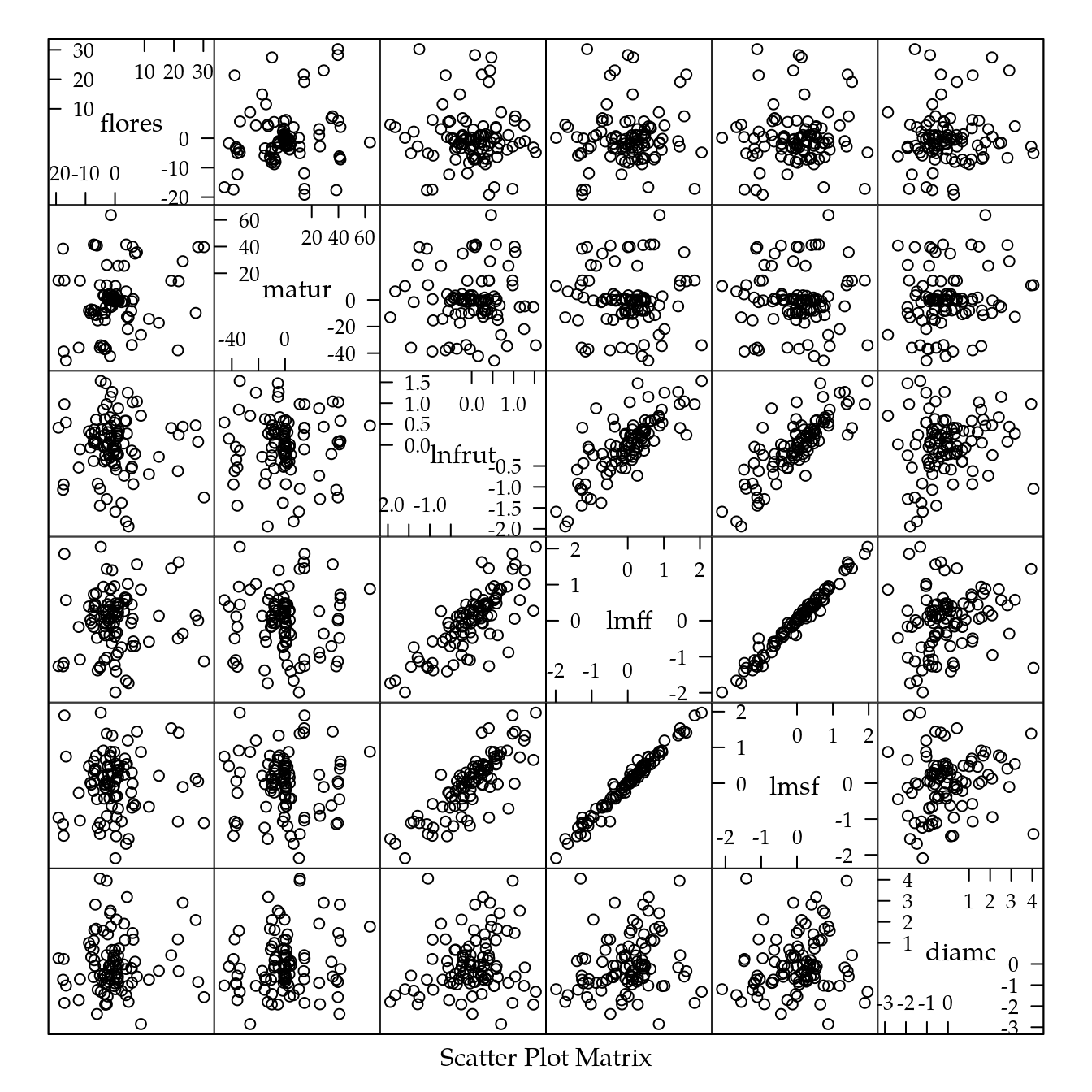
cor(r)## flores matur lnfrut lmff
## flores 1.00000000 0.186289363 -0.05533574 0.05587337
## matur 0.18628936 1.000000000 0.01203903 -0.02458323
## lnfrut -0.05533574 0.012039029 1.00000000 0.77766165
## lmff 0.05587337 -0.024583227 0.77766165 1.00000000
## lmsf 0.03264835 -0.008338419 0.81572752 0.98677552
## diamc 0.06912871 0.146172538 0.17445501 0.17448815
## lmsf diamc
## flores 0.032648355 0.06912871
## matur -0.008338419 0.14617254
## lnfrut 0.815727524 0.17445501
## lmff 0.986775515 0.17448815
## lmsf 1.000000000 0.14857934
## diamc 0.148579336 1.00000000# Gráfico de correlação.
corrplot::corrplot(cor(r),
type = "upper",
tl.pos = "d",
outline = TRUE,
method = "ellipse")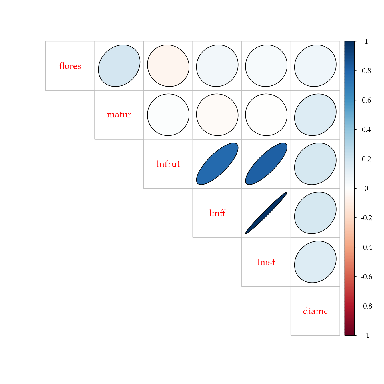
#-----------------------------------------------------------------------
# Canonical discriminant analysis.

# Efeito de genótipo.
cdg <- candisc(m1, term = "gen")
cdg
##
## Canonical Discriminant Analysis for gen:
##
## CanRsq Eigenvalue Difference Percent Cumulative
## 1 0.854204 5.858885 2.2482 43.75537 43.755
## 2 0.783111 3.610653 2.2482 26.96511 70.720
## 3 0.738581 2.825280 2.2482 21.09978 91.820
## 4 0.467773 0.878898 2.2482 6.56379 98.384
## 5 0.149359 0.175585 2.2482 1.31130 99.695
## 6 0.039194 0.040793 2.2482 0.30465 100.000
##
## Test of H0: The canonical correlations in the
## current row and all that follow are zero
##
## LR test stat approx F numDF denDF Pr(> F)
## 1 0.00360 21.9518 42 397.45 < 2.2e-16 ***
## 2 0.02466 17.3668 30 342.00 < 2.2e-16 ***
## 3 0.11371 13.2518 20 286.18 < 2.2e-16 ***
## 4 0.43499 7.1015 12 230.47 5.584e-11 ***
## 5 0.81730 3.1134 6 176.00 0.00635 **
## 6 0.96081 2
## ---
## Signif. codes: 0 '***' 0.001 '**' 0.01 '*' 0.05 '.' 0.1 ' ' 1par(mfrow = c(2, 2))
plot(cdg)
plot(cdg, which = c(1, 3))
plot(cdg, which = c(2, 3))
plot(cdg, which = c(1, 4))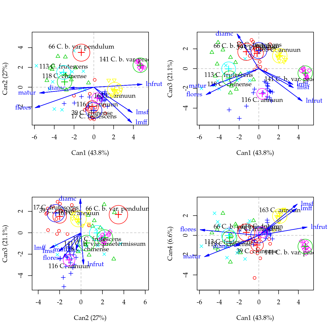
layout(1)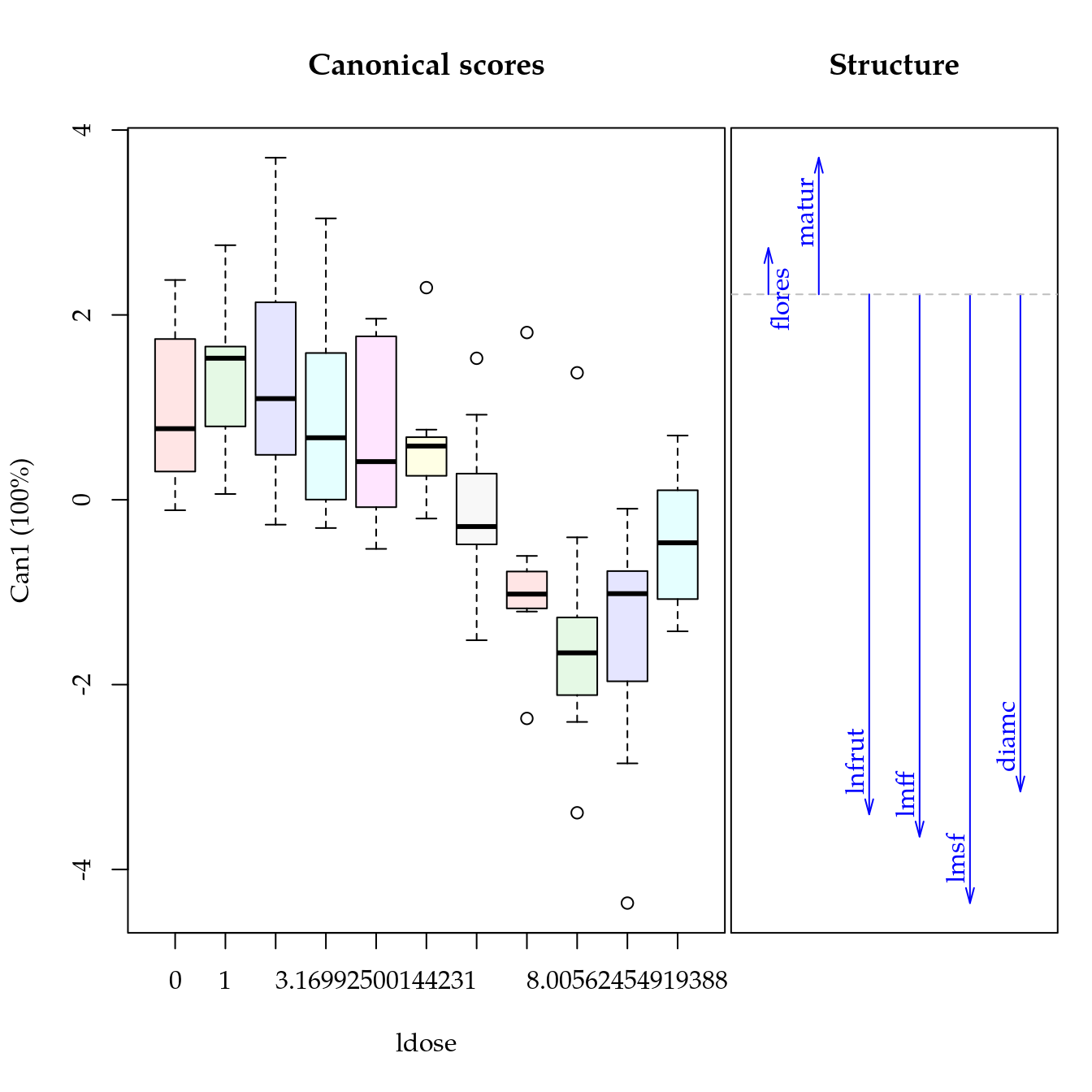
cdd##
## Canonical Discriminant Analysis for ldose:
##
## CanRsq Eigenvalue Difference Percent Cumulative
## 1 0.51933 1.0804 100 100
##
## Test of H0: The canonical correlations in the
## current row and all that follow are zero
##
## LR test stat approx F numDF denDF Pr(> F)
## 1 0.48067 16.206 6 90 1.464e-12 ***
## ---
## Signif. codes: 0 '***' 0.001 '**' 0.01 '*' 0.05 '.' 0.1 ' ' 1Variáveis de fruto
# Estrutura dos dados.
str(cn$fruto)
## 'data.frame': 451 obs. of 7 variables:
## $ gen : Factor w/ 8 levels "39 C. chinense",..: 1 1 1 1 1 1 1 1 1 1 ...
## $ dose : int 0 0 0 0 0 1 1 16 32 64 ...
## $ rept : int 1 1 1 1 1 1 1 1 1 1 ...
## $ fruto: int 1 2 3 4 5 1 2 1 1 1 ...
## $ diamf: num 19 18 23 25 19 27 29 45 46 36 ...
## $ compf: num 11.9 10.9 14.2 13.5 12.4 ...
## $ genab: Factor w/ 8 levels "39 chi","118 chi",..: 1 1 1 1 1 1 1 1 1 1 ...# Log da dose será usado nas análises.
cn$fruto$ldose <- log2(cn$fruto$dose + 1)
# Frequência dos dados.
xtabs(~genab + dose, data = cn$fruto)## dose
## genab 0 1 2 4 8 16 32 64 128 256 512
## 39 chi 5 5 0 0 2 6 6 10 10 10 10
## 118 chi 4 2 3 6 1 8 10 8 10 10 0
## 17 fru 1 0 2 0 3 5 5 5 5 5 2
## 113 fru 6 7 0 3 4 3 2 5 10 5 0
## 116 ann 10 5 10 10 10 10 10 10 10 10 10
## 163 ann 5 5 5 5 5 5 5 5 5 5 5
## 66 pen 0 2 1 4 5 0 5 5 5 5 0
## 141 pra 5 5 5 5 5 5 5 5 5 5 5# Agregando os dados para os valores médios e total de observações.
dc <- ddply(.data = cn$fruto,
.variables = .(genab, ldose, rept),
.fun = summarise,
diamf = mean(diamf, na.rm = TRUE),
compf = mean(compf, na.rm = TRUE),
n = max(fruto))
str(dc)## 'data.frame': 108 obs. of 6 variables:
## $ genab: Factor w/ 8 levels "39 chi","118 chi",..: 1 1 1 1 1 1 1 1 1 1 ...
## $ ldose: num 0 1 1 3.17 4.09 ...
## $ rept : int 1 1 2 2 1 2 1 2 1 2 ...
## $ diamf: num 20.8 28 31 30 45 23.2 46 21.2 29.4 35.2 ...
## $ compf: num 12.6 21 20.2 13.2 20 ...
## $ n : int 5 2 3 2 1 5 1 5 5 5 ...xyplot(diamf + compf ~ ldose | genab,
scales = list(y = list(log = 10)),
data = dc) +
glayer(panel.smoother(x, y,
method = "lm",
form = y ~ poly(x, degree = 2), ...))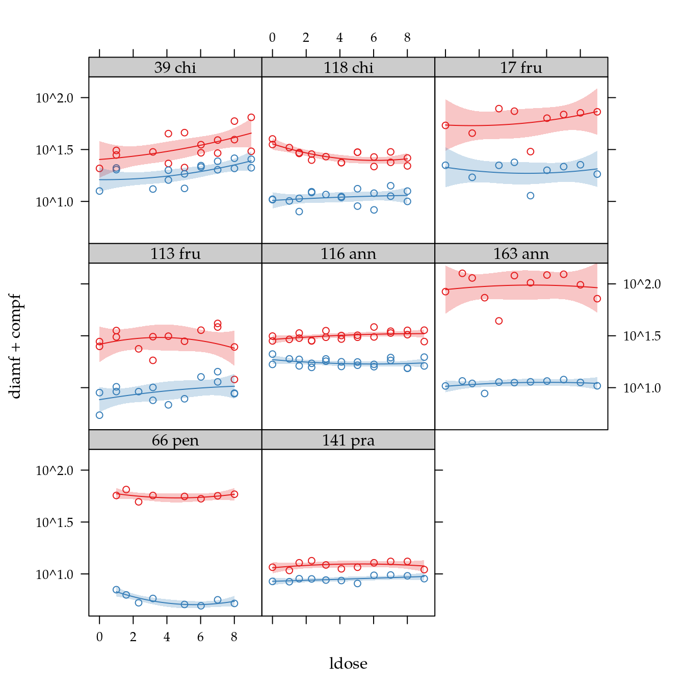
Comprimento dos frutos
# Declara modelo fatorial com dose expresso por polinômio de grau 2.
m0 <- lm(log10(compf) ~ genab * poly(ldose, degree = 2),
         data = dc,
         weights = n)
anova(m0)
## Analysis of Variance Table
##
## Response: log10(compf)
## Df Sum Sq Mean Sq F value Pr(>F)
## genab 7 12.0141 1.71631 95.9964 < 2e-16
## poly(ldose, degree = 2) 2 0.1351 0.06757 3.7795 0.02681
## genab:poly(ldose, degree = 2) 14 0.3762 0.02687 1.5030 0.12783
## Residuals 84 1.5018 0.01788
##
## genab ***
## poly(ldose, degree = 2) *
## genab:poly(ldose, degree = 2)
## Residuals
## ---
## Signif. codes: 0 '***' 0.001 '**' 0.01 '*' 0.05 '.' 0.1 ' ' 1# par(mfrow = c(2, 2))
# plot(m0); layout(1)
# MASS::boxcox(m0)
# Declara o modelo reduzido contendo apenas o efeito de genótipo.
m1 <- update(m0, . ~ genab + ldose)
anova(m1, m0)## Analysis of Variance Table
##
## Model 1: log10(compf) ~ genab + ldose
## Model 2: log10(compf) ~ genab * poly(ldose, degree = 2)
## Res.Df RSS Df Sum of Sq F Pr(>F)
## 1 99 1.8876
## 2 84 1.5018 15 0.38574 1.4384 0.1488# Predição.
pred <- with(da,
expand.grid(genab = levels(genab),
ldose = seq(min(ldose),
max(ldose),
length.out = 30),
KEEP.OUT.ATTRS = FALSE))
ci <- predict(m1, newdata = pred, interval = "confidence")
pred <- cbind(pred, as.data.frame(ci))
# Gráfico dos resultados.
xyplot(log10(compf) ~ ldose | genab,
data = dc,
xlab = labs$xlab,
ylab = "Comprimento do fruto (mm, log 10)") +
as.layer(
xyplot(fit + lwr + upr ~ ldose | genab,
col = c("black", "gray", "gray"),
data = pred,
type = "l"))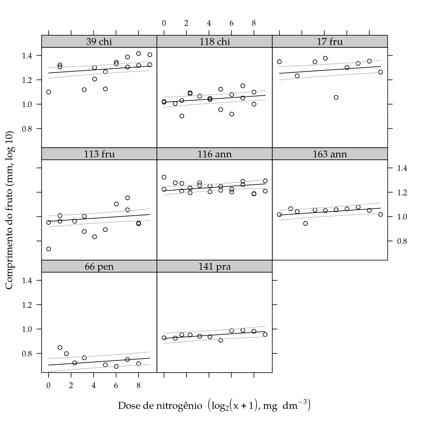
Diâmetro dos frutos
# Declara modelo fatorial com dose expresso por polinômio de grau 2.
m0 <- lm(log10(diamf) ~ genab * poly(ldose, degree = 2),
         data = dc,
         weights = n)
anova(m0)
## Analysis of Variance Table
##
## Response: log10(diamf)
## Df Sum Sq Mean Sq F value Pr(>F)
## genab 7 26.1467 3.7352 94.2446 <2e-16 ***
## poly(ldose, degree = 2) 2 0.1805 0.0902 2.2768 0.1089
## genab:poly(ldose, degree = 2) 14 0.6999 0.0500 1.2614 0.2489
## Residuals 84 3.3292 0.0396
## ---
## Signif. codes: 0 '***' 0.001 '**' 0.01 '*' 0.05 '.' 0.1 ' ' 1# par(mfrow = c(2, 2))
# plot(m0); layout(1)
# MASS::boxcox(m0)
# Declara o modelo reduzido contendo apenas o efeito de genótipo.
m1 <- update(m0, . ~ genab + ldose)
anova(m1, m0)## Analysis of Variance Table
##
## Model 1: log10(diamf) ~ genab + ldose
## Model 2: log10(diamf) ~ genab * poly(ldose, degree = 2)
## Res.Df RSS Df Sum of Sq F Pr(>F)
## 1 99 4.0495
## 2 84 3.3292 15 0.72026 1.2115 0.2796# Predição.
pred <- with(da,
expand.grid(genab = levels(genab),
ldose = seq(min(ldose),
max(ldose),
length.out = 30),
KEEP.OUT.ATTRS = FALSE))
ci <- predict(m1, newdata = pred, interval = "confidence")
pred <- cbind(pred, as.data.frame(ci))
# Gráfico dos resultados.
xyplot(log10(diamf) ~ ldose | genab,
data = dc,
xlab = labs$xlab,
ylab = "Comprimento do fruto (mm, log 10)") +
as.layer(
xyplot(fit + lwr + upr ~ ldose | genab,
col = c("black", "gray", "gray"),
data = pred,
type = "l"))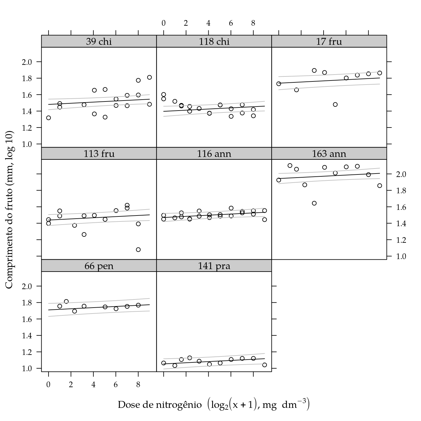
Análise canônica discriminante
#-----------------------------------------------------------------------
# Análise multivariada.

# ATTENTION: o argumento `weights` não tem utilidade quando o lado
# esquerdo da fórmula é uma matriz. Com isso, não é possível ponderar
# análises multivariadas.

# Modelos multivariado usando o log das variáveis.
m0 <- lm(cbind(ldiamf = log10(diamf),
               lcompf = log10(compf)) ~
             genab * (ldose + I(ldose^2)),
         data = dc)
anova(m0)
## Analysis of Variance Table
##
## Df Pillai approx F num Df den Df Pr(>F)
## (Intercept) 1 0.99761 17325.5 2 83 < 2.2e-16 ***
## genab 7 1.75789 87.1 14 168 < 2.2e-16 ***
## ldose 1 0.05564 2.4 2 83 0.092961 .
## I(ldose^2) 1 0.00736 0.3 2 83 0.736069
## genab:ldose 7 0.33649 2.4 14 168 0.003969 **
## genab:I(ldose^2) 7 0.06866 0.4 14 168 0.964533
## Residuals 84
## ---
## Signif. codes: 0 '***' 0.001 '**' 0.01 '*' 0.05 '.' 0.1 ' ' 1## Analysis of Variance Table
##
## Model 1: cbind(ldiamf = log10(diamf), lcompf = log10(compf)) ~ genab +
## ldose + genab:ldose
## Model 2: cbind(ldiamf = log10(diamf), lcompf = log10(compf)) ~ genab *
## (ldose + I(ldose^2))
## Res.Df Df Gen.var. Pillai approx F num Df den Df Pr(>F)
## 1 92 0.0058236
## 2 84 -8 0.0061319 0.077257 0.4219 16 168 0.9753anova(m1)## Analysis of Variance Table
##
## Df Pillai approx F num Df den Df Pr(>F)
## (Intercept) 1 0.99751 18250.1 2 91 < 2.2e-16 ***
## genab 7 1.74947 91.8 14 184 < 2.2e-16 ***
## ldose 1 0.05364 2.6 2 91 0.081386 .
## genab:ldose 7 0.32515 2.6 14 184 0.002291 **
## Residuals 92
## ---
## Signif. codes: 0 '***' 0.001 '**' 0.01 '*' 0.05 '.' 0.1 ' ' 1# r <- residuals(m1)
# splom(r, as.matrix = TRUE)
# cor(r)
#-----------------------------------------------------------------------
# Análise canonica discriminante.
# Efeito de genótipo.
cdg <- candisc(m1, term = "genab")
plot(cdg)## Vector scale factor set to 7.521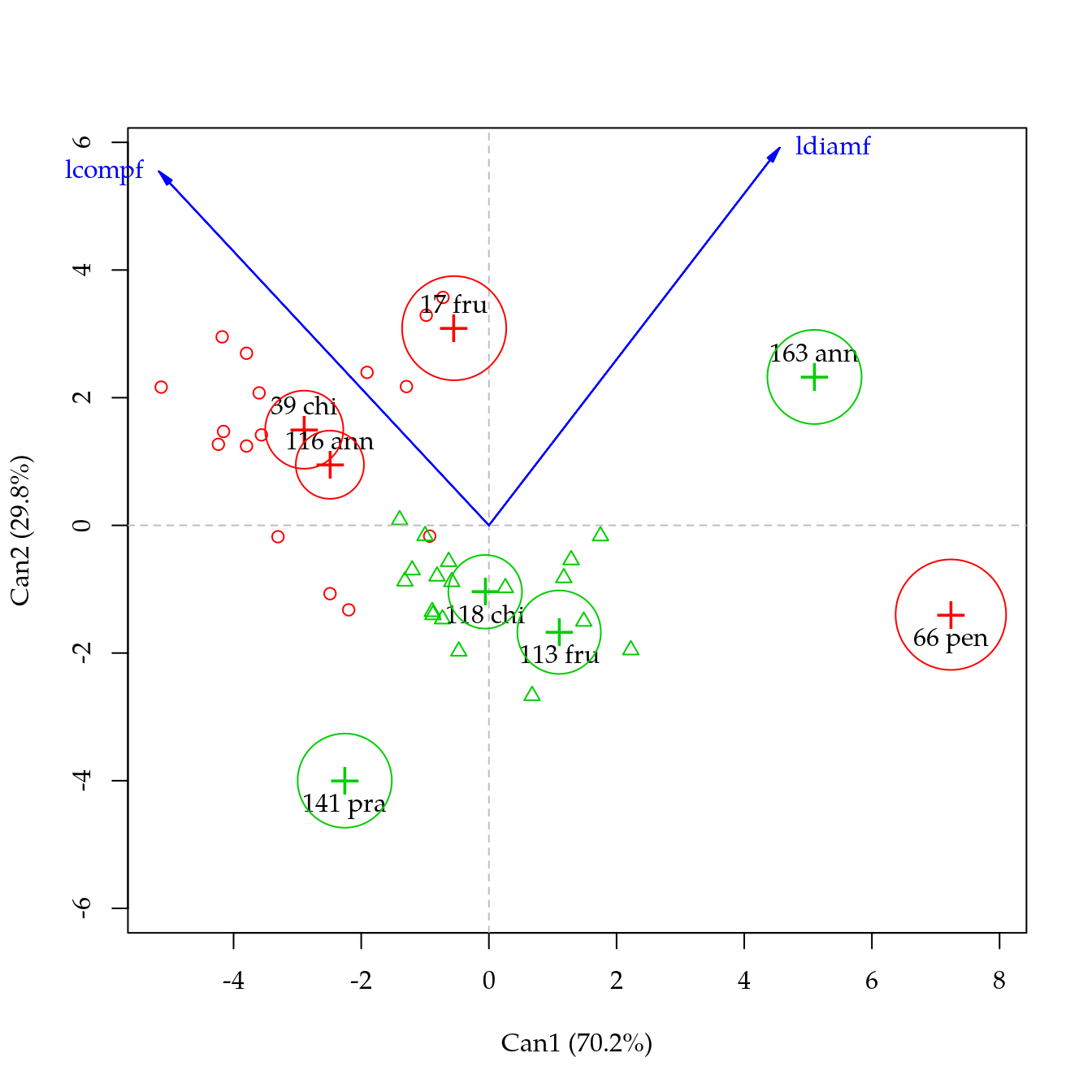
cdg##
## Canonical Discriminant Analysis for genab:
##
## CanRsq Eigenvalue Difference Percent Cumulative
## 1 0.91844 11.2604 6.4796 70.197 70.197
## 2 0.82701 4.7808 6.4796 29.803 100.000
##
## Test of H0: The canonical correlations in the
## current row and all that follow are zero
##
## LR test stat approx F numDF denDF Pr(> F)
## 1 0.014109 104.92 14 198 < 2.2e-16 ***
## 2 0.172986 79.68 6 100 < 2.2e-16 ***
## ---
## Signif. codes: 0 '***' 0.001 '**' 0.01 '*' 0.05 '.' 0.1 ' ' 1summary(cdg)##
## Canonical Discriminant Analysis for genab:
##
## CanRsq Eigenvalue Difference Percent Cumulative
## 1 0.91844 11.2604 6.4796 70.197 70.197
## 2 0.82701 4.7808 6.4796 29.803 100.000
##
## Class means:
##
## Can1 Can2
## 39 chi -2.892798 1.49917
## 118 chi -0.058567 -1.04014
## 17 fru -0.544192 3.08913
## 113 fru 1.099827 -1.67311
## 116 ann -2.491246 0.95019
## 163 ann 5.100420 2.32559
## 66 pen 7.237019 -1.39902
## 141 pra -2.258680 -3.99874
##
## std coefficients:
## Can1 Can2
## ldiamf 0.95855 0.61929
## lcompf -1.00450 0.54157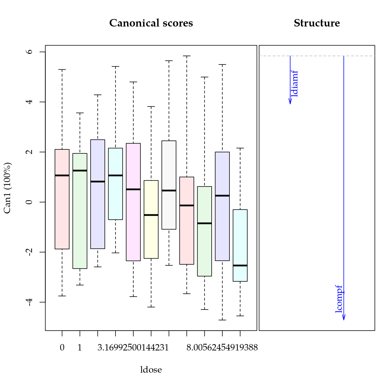
cdl##
## Canonical Discriminant Analysis for ldose:
##
## CanRsq Eigenvalue Difference Percent Cumulative
## 1 0.053641 0.056681 100 100
##
## Test of H0: The canonical correlations in the
## current row and all that follow are zero
##
## LR test stat approx F numDF denDF Pr(> F)
## 1 0.94636 2summary(cdl)##
## Canonical Discriminant Analysis for ldose:
##
## CanRsq Eigenvalue Difference Percent Cumulative
## 1 0.053641 0.056681 100 100
##
## Class means:
##
## [1] 0.421001 0.215502 0.574274 1.053035 0.362274 -0.428709
## [7] 0.658452 -0.277968 -0.829023 -0.073323 -1.694403
##
## std coefficients:
## ldiamf lcompf
## -0.020525 -0.989949Teores de substâncias nos frutos
# Estrutura dos dados.
str(cn$teor)
## 'data.frame': 217 obs. of 10 variables:
## $ gen : Factor w/ 8 levels "39 C. chinense",..: 1 1 1 1 1 1 1 1 1 1 ...
## $ dose : int 0 0 0 16 16 16 256 256 256 1 ...
## $ rept : int 1 1 1 1 1 1 1 1 1 2 ...
## $ ddph : num 34.4 35.3 34.4 22.3 23.2 ...
## $ lico : num 0.57 0.48 0.46 0.08 0.38 0.02 NA NA NA 0.06 ...
## $ bcaro : num 1.35 1.28 1.22 0 0 0.04 NA NA NA 0 ...
## $ polifen: num 151 154 156 118 106 ...
## $ flavon : num 35.1 48.7 20.2 NA NA ...
## $ antoc : num 21.08 19.37 6.51 NA NA ...
## $ genab : Factor w/ 8 levels "39 chi","118 chi",..: 1 1 1 1 1 1 1 1 1 1 ...# Frequência dos dados.
xtabs(~genab + dose, data = cn$teor)## dose
## genab 0 1 2 4 8 16 32 64 128 256 512
## 39 chi 3 3 0 0 0 6 3 5 4 6 0
## 118 chi 6 3 0 3 0 6 6 6 6 6 0
## 17 fru 0 0 0 0 0 3 3 3 3 3 0
## 113 fru 3 6 0 3 3 0 6 4 3 0 0
## 116 ann 6 0 3 6 3 6 6 6 6 6 3
## 163 ann 3 3 3 3 3 3 3 3 3 3 0
## 66 pen 0 0 0 0 0 0 0 0 0 0 0
## 141 pra 3 0 0 0 3 3 3 3 3 3 0# Agrega para as médias das replicadas (são 3).
dd <- ddply(.data = cn$teor,
.variables = .(genab, dose, rept),
.fun = colwise(mean, is.numeric))
str(dd)## 'data.frame': 71 obs. of 9 variables:
## $ genab : Factor w/ 8 levels "39 chi","118 chi",..: 1 1 1 1 1 1 1 1 1 2 ...
## $ dose : int 0 1 16 16 32 64 128 256 256 0 ...
## $ rept : int 1 2 1 2 2 2 2 1 2 1 ...
## $ ddph : num 34.7 34.3 23.3 22.5 21.2 ...
## $ lico : num 0.5033 0.0333 0.16 0.44 0.4167 ...
## $ bcaro : num 1.2833 0.0133 0.0133 0.9533 0.9367 ...
## $ polifen: num 154 111 118 186 116 ...
## $ flavon : num 34.7 10.2 NA NA 21 ...
## $ antoc : num 15.653 0.533 NA NA 8.163 ...# Log da dose será usada nas análises.
dd$ldose <- log2(dd$dose + 1)DDPH
# Exploratória.
xyplot(log10(ddph) ~ ldose | genab,
       data = dd) +
    layer(panel.smoother(x, y,
                         method = "lm",
                         form = y ~ poly(x, degree = 2), ...))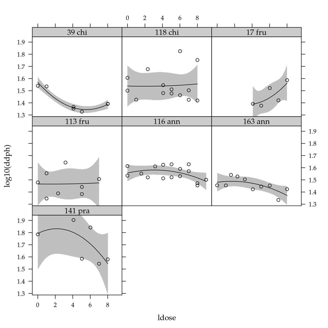
# Declara modelo fatorial com dose expresso por polinômio de grau 2.
m0 <- lm(log10(ddph) ~ genab * poly(ldose, degree = 2),
         data = dd)
anova(m0)
## Analysis of Variance Table
##
## Response: log10(ddph)
## Df Sum Sq Mean Sq F value Pr(>F)
## genab 6 0.39308 0.065513 7.0983 2.312e-05
## poly(ldose, degree = 2) 2 0.02522 0.012612 1.3664 0.2654
## genab:poly(ldose, degree = 2) 12 0.11411 0.009509 1.0303 0.4389
## Residuals 45 0.41533 0.009229
##
## genab ***
## poly(ldose, degree = 2)
## genab:poly(ldose, degree = 2)
## Residuals
## ---
## Signif. codes: 0 '***' 0.001 '**' 0.01 '*' 0.05 '.' 0.1 ' ' 1# par(mfrow = c(2, 2))
# plot(m0); layout(1)
# MASS::boxcox(m0)
# Declara o modelo reduzido contendo apenas o efeito de genótipo.
m1 <- update(m0, . ~ genab)
anova(m1, m0)## Analysis of Variance Table
##
## Model 1: log10(ddph) ~ genab
## Model 2: log10(ddph) ~ genab * poly(ldose, degree = 2)
## Res.Df RSS Df Sum of Sq F Pr(>F)
## 1 59 0.55466
## 2 45 0.41533 14 0.13933 1.0783 0.4013# Comparações múltiplas entre médias de genótipos.
L <- LE_matrix(m1, effect = "genab")
rownames(L) <- attr(L, "grid")$genab
pred <- apmc(L, m1, "genab", test = "fdr")
arrange(pred, -fit)## genab fit lwr upr cld
## 1 141 pra 1.706592 1.627386 1.785798 a
## 2 116 ann 1.553944 1.505441 1.602448 b
## 3 118 chi 1.543566 1.491714 1.595419 bc
## 4 113 fru 1.467836 1.399241 1.536430 bd
## 5 17 fru 1.459445 1.372679 1.546210 bd
## 6 163 ann 1.456009 1.394657 1.517361 cd
## 7 39 chi 1.415070 1.341739 1.488400 d# Gráfico de segmentos.
segplot(reorder(genab, fit) ~ lwr + upr,
centers = fit,
data = pred,
cld = sprintf("%0.2f %s", pred$fit, pred$cld),
draw = FALSE,
xlab = "DDPH (mg/100 g) (log 10)",
ylab = "Genótipo de pimenta") +
layer(panel.text(x = centers,
y = z,
labels = cld,
pos = 3))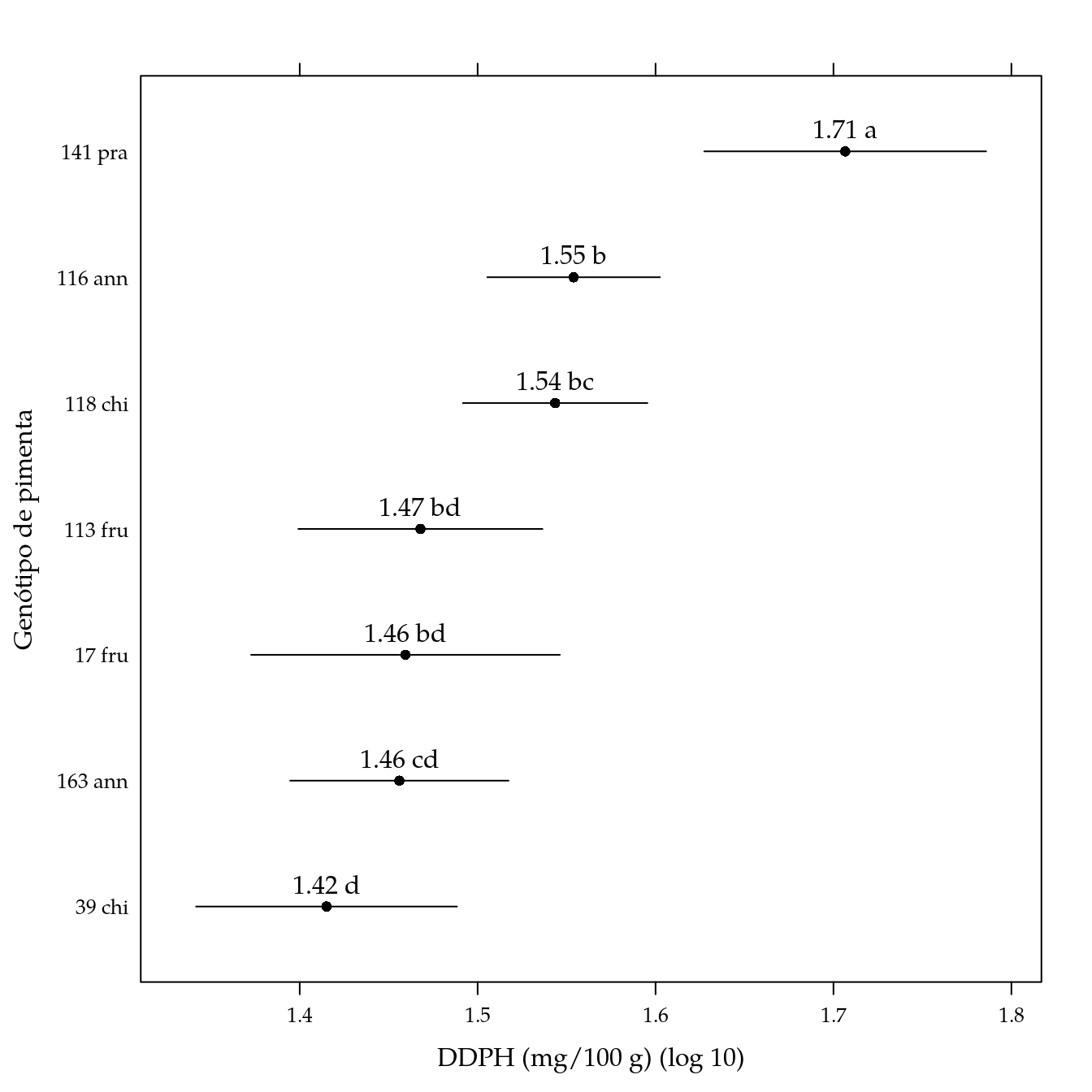
Licofenol
# Exploratória.
xyplot(lico ~ ldose | genab,
       data = dd) +
    layer(panel.smoother(x, y,
                         method = "lm",
                         form = y ~ poly(x, degree = 2), ...))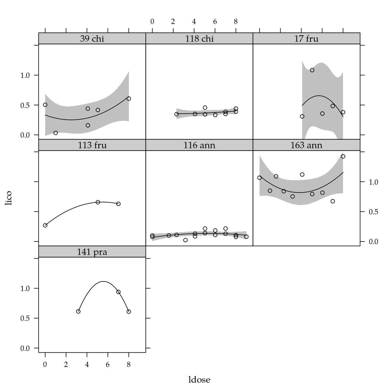
# Declara modelo fatorial com dose expresso por polinômio de grau 2.
m0 <- lm(lico ~ genab * poly(ldose, degree = 2),
         data = dd)
anova(m0)
## Analysis of Variance Table
##
## Response: lico
## Df Sum Sq Mean Sq F value Pr(>F)
## genab 6 4.5481 0.75802 27.3225 4.384e-11
## poly(ldose, degree = 2) 2 0.0545 0.02725 0.9821 0.3859
## genab:poly(ldose, degree = 2) 12 0.4188 0.03490 1.2580 0.2910
## Residuals 31 0.8600 0.02774
##
## genab ***
## poly(ldose, degree = 2)
## genab:poly(ldose, degree = 2)
## Residuals
## ---
## Signif. codes: 0 '***' 0.001 '**' 0.01 '*' 0.05 '.' 0.1 ' ' 1# par(mfrow = c(2, 2))
# plot(m0); layout(1)
# MASS::boxcox(m0)
# Declara o modelo reduzido contendo apenas o efeito de genótipo.
m1 <- update(m0, . ~ genab)
anova(m1, m0)## Analysis of Variance Table
##
## Model 1: lico ~ genab
## Model 2: lico ~ genab * poly(ldose, degree = 2)
## Res.Df RSS Df Sum of Sq F Pr(>F)
## 1 45 1.33337
## 2 31 0.86004 14 0.47332 1.2186 0.3114# Comparações múltiplas entre médias de genótipos.
L <- LE_matrix(m1, effect = "genab")
rownames(L) <- attr(L, "grid")$genab
pred <- apmc(L, m1, "genab", test = "fdr")
arrange(pred, -fit)## genab fit lwr upr cld
## 1 163 ann 0.9426667 0.83303138 1.0523020 a
## 2 141 pra 0.7211111 0.52094537 0.9212768 ab
## 3 17 fru 0.5226667 0.36761895 0.6777144 bc
## 4 113 fru 0.5188889 0.31872315 0.7190546 bc
## 5 118 chi 0.3774074 0.26184166 0.4929732 c
## 6 39 chi 0.3600000 0.21846145 0.5015386 c
## 7 116 ann 0.1179167 0.03124236 0.2045910 d# Gráfico de segmentos.
segplot(reorder(genab, fit) ~ lwr + upr,
centers = fit,
data = pred,
cld = sprintf("%0.2f %s", pred$fit, pred$cld),
draw = FALSE,
xlab = "Licofenol (mg/100 g)",
ylab = "Genótipo de pimenta") +
layer(panel.text(x = centers,
y = z,
labels = cld,
pos = 3))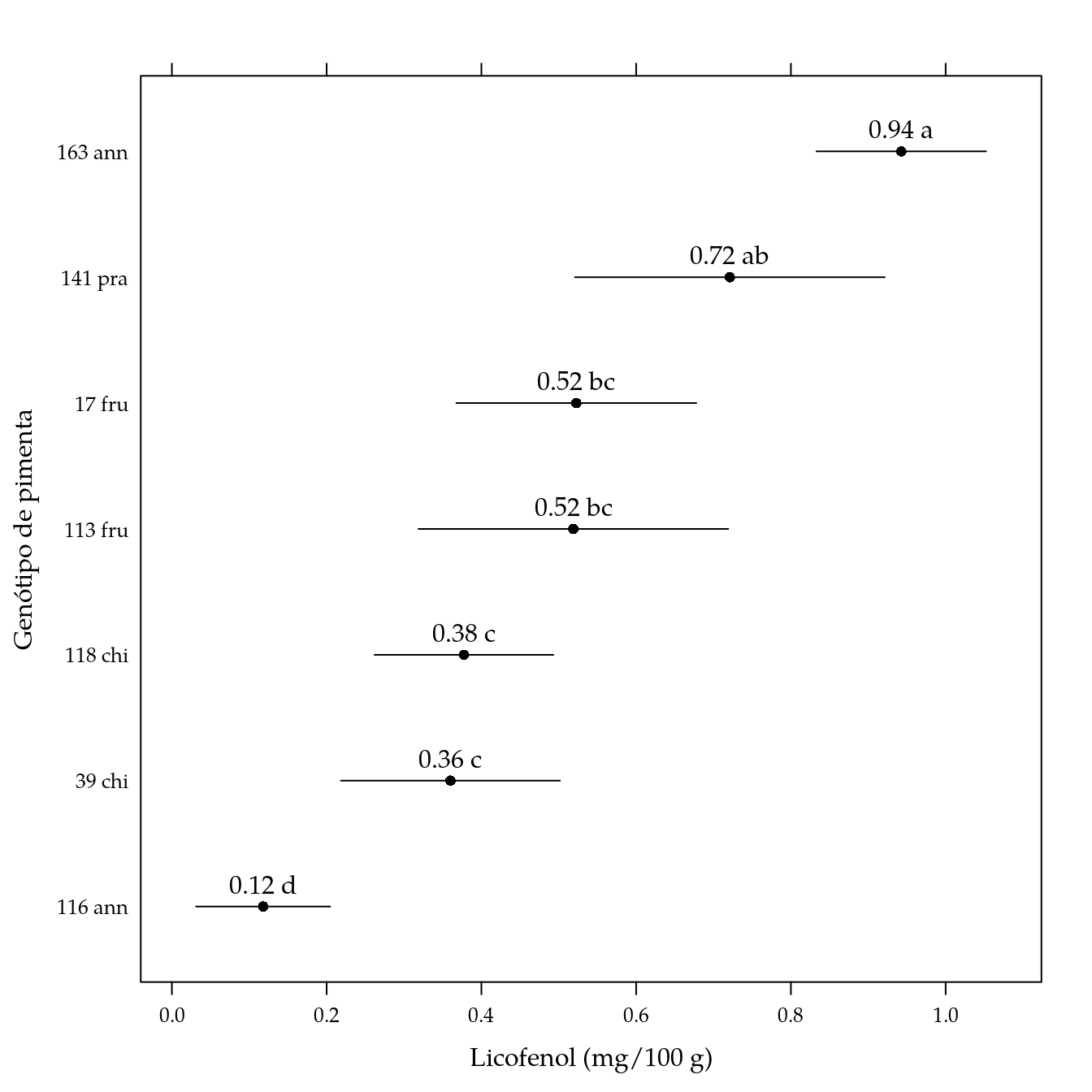
\(\beta\)-caroteno
# Exploratória.
xyplot(bcaro ~ ldose | genab,
       data = dd) +
    layer(panel.smoother(x, y,
                         method = "lm",
                         form = y ~ poly(x, degree = 2), ...))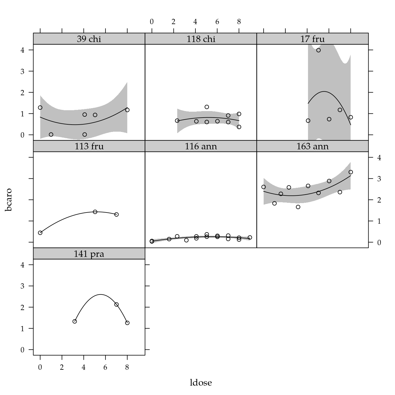
# Declara modelo fatorial com dose expresso por polinômio de grau 2.
m0 <- lm(bcaro ~ genab * poly(ldose, degree = 2),
         data = dd)
anova(m0)
## Analysis of Variance Table
##
## Response: bcaro
## Df Sum Sq Mean Sq F value Pr(>F)
## genab 6 34.162 5.6937 18.5963 4.892e-09
## poly(ldose, degree = 2) 2 0.530 0.2649 0.8651 0.4309
## genab:poly(ldose, degree = 2) 12 3.475 0.2896 0.9458 0.5170
## Residuals 31 9.491 0.3062
##
## genab ***
## poly(ldose, degree = 2)
## genab:poly(ldose, degree = 2)
## Residuals
## ---
## Signif. codes: 0 '***' 0.001 '**' 0.01 '*' 0.05 '.' 0.1 ' ' 1# par(mfrow = c(2, 2))
# plot(m0); layout(1)
# MASS::boxcox(m0)
# Declara o modelo reduzido contendo apenas o efeito de genótipo.
m1 <- update(m0, . ~ genab)
anova(m1, m0)## Analysis of Variance Table
##
## Model 1: bcaro ~ genab
## Model 2: bcaro ~ genab * poly(ldose, degree = 2)
## Res.Df RSS Df Sum of Sq F Pr(>F)
## 1 45 13.4960
## 2 31 9.4914 14 4.0045 0.9342 0.5356# Comparações múltiplas entre médias de genótipos.
L <- LE_matrix(m1, effect = "genab")
rownames(L) <- attr(L, "grid")$genab
pred <- apmc(L, m1, "genab", test = "fdr")
arrange(pred, -fit)## genab fit lwr upr cld
## 1 163 ann 2.4480000 2.09919902 2.7968010 a
## 2 141 pra 1.5722222 0.93540167 2.2090428 bc
## 3 17 fru 1.4780000 0.98472092 1.9712791 b
## 4 113 fru 1.0600000 0.42317945 1.6968206 bd
## 5 118 chi 0.7470370 0.37936852 1.1147056 d
## 6 39 chi 0.7283333 0.27803320 1.1786335 cde
## 7 116 ann 0.2043750 -0.07137639 0.4801264 e# Gráfico de segmentos.
segplot(reorder(genab, fit) ~ lwr + upr,
centers = fit,
data = pred,
cld = sprintf("%0.2f %s", pred$fit, pred$cld),
draw = FALSE,
xlab = "beta-caroteno (mg/100 g)",
ylab = "Genótipo de pimenta") +
layer(panel.text(x = centers,
y = z,
labels = cld,
pos = 3))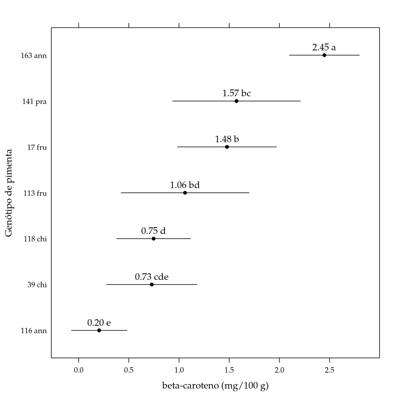
Polifenol
# Exploratória.
xyplot(polifen ~ ldose | genab,
       data = dd) +
    layer(panel.smoother(x, y,
                         method = "lm",
                         form = y ~ poly(x, degree = 2), ...))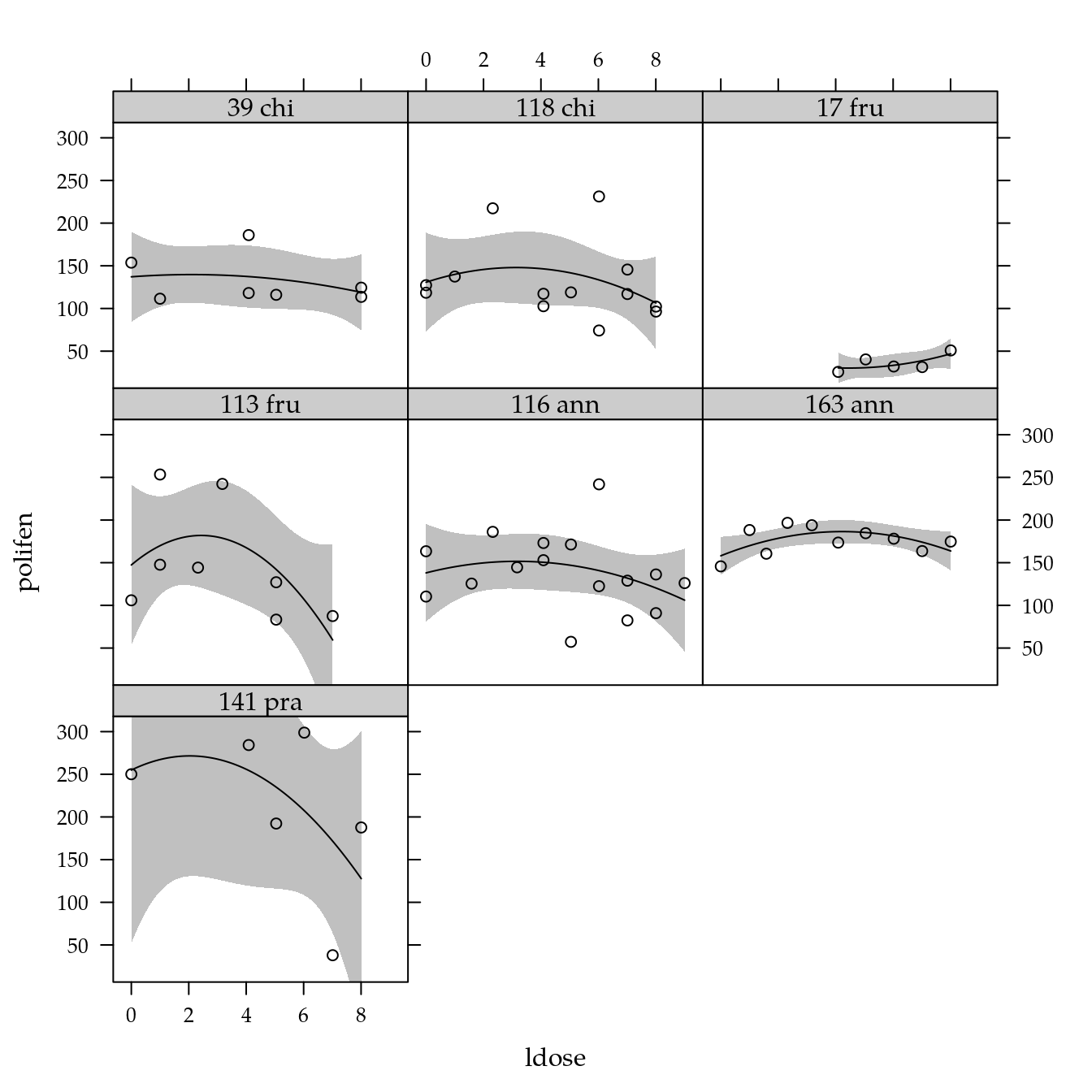
# Declara modelo fatorial com dose expresso por polinômio de grau 2.
m0 <- lm(polifen ~ genab * poly(ldose, degree = 2),
         data = dd)
anova(m0)
## Analysis of Variance Table
##
## Response: polifen
## Df Sum Sq Mean Sq F value Pr(>F)
## genab 6 97073 16178.8 6.6778 4.496e-05
## poly(ldose, degree = 2) 2 12490 6245.2 2.5777 0.08738
## genab:poly(ldose, degree = 2) 12 17789 1482.5 0.6119 0.82042
## Residuals 44 106602 2422.8
##
## genab ***
## poly(ldose, degree = 2) .
## genab:poly(ldose, degree = 2)
## Residuals
## ---
## Signif. codes: 0 '***' 0.001 '**' 0.01 '*' 0.05 '.' 0.1 ' ' 1# par(mfrow = c(2, 2))
# plot(m0); layout(1)
# MASS::boxcox(m0)
# Declara o modelo reduzido contendo apenas o efeito de genótipo.
m1 <- update(m0, . ~ genab)
anova(m1, m0)## Analysis of Variance Table
##
## Model 1: polifen ~ genab
## Model 2: polifen ~ genab * poly(ldose, degree = 2)
## Res.Df RSS Df Sum of Sq F Pr(>F)
## 1 58 136882
## 2 44 106602 14 30280 0.8927 0.5719# Comparações múltiplas entre médias de genótipos.
L <- LE_matrix(m1, effect = "genab")
rownames(L) <- attr(L, "grid")$genab
pred <- apmc(L, m1, "genab", test = "fdr")
arrange(pred, -fit)## genab fit lwr upr cld
## 1 141 pra 208.51111 168.811466 248.21076 a
## 2 163 ann 175.98400 145.232787 206.73521 ab
## 3 113 fru 148.93458 114.553682 183.31548 ab
## 4 116 ann 138.35333 114.042365 162.66430 b
## 5 39 chi 131.88190 95.127175 168.63663 b
## 6 118 chi 131.20692 104.236325 158.17752 b
## 7 17 fru 36.02533 -7.463449 79.51412 c# Gráfico de segmentos.
segplot(reorder(genab, fit) ~ lwr + upr,
centers = fit,
data = pred,
cld = sprintf("%0.2f %s", pred$fit, pred$cld),
draw = FALSE,
xlab = "Polifenol (mg/100 g)",
ylab = "Genótipo de pimenta") +
layer(panel.text(x = centers,
y = z,
labels = cld,
pos = 3))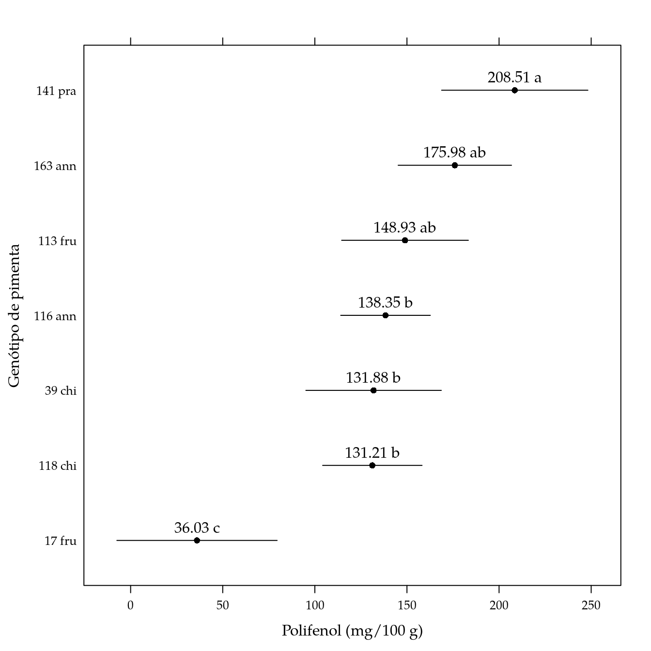
Flavonol
# Exploratória.
xyplot(flavon ~ ldose | genab,
       data = dd) +
    layer(panel.smoother(x, y,
                         method = "lm",
                         form = y ~ poly(x, degree = 2), ...))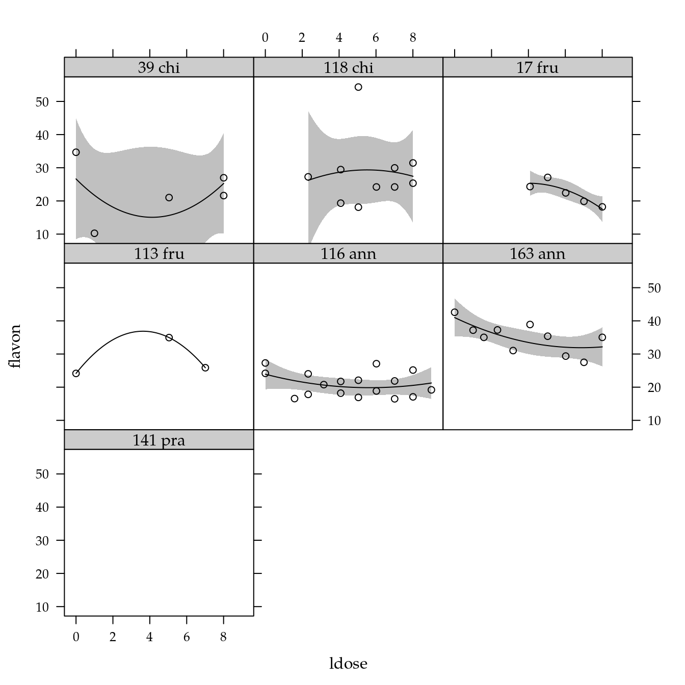
# Declara modelo fatorial com dose expresso por polinômio de grau 2.
m0 <- lm(flavon ~ genab * poly(ldose, degree = 2),
         data = dd)
anova(m0)
## Analysis of Variance Table
##
## Response: flavon
## Df Sum Sq Mean Sq F value Pr(>F)
## genab 5 1424.02 284.804 6.3156 0.0003493
## poly(ldose, degree = 2) 2 49.51 24.757 0.5490 0.5828703
## genab:poly(ldose, degree = 2) 10 263.89 26.389 0.5852 0.8137673
## Residuals 32 1443.05 45.095
##
## genab ***
## poly(ldose, degree = 2)
## genab:poly(ldose, degree = 2)
## Residuals
## ---
## Signif. codes: 0 '***' 0.001 '**' 0.01 '*' 0.05 '.' 0.1 ' ' 1# par(mfrow = c(2, 2))
# plot(m0); layout(1)
# MASS::boxcox(m0)
# Declara o modelo reduzido contendo apenas o efeito de genótipo.
m1 <- update(m0, . ~ genab)
anova(m1, m0)## Analysis of Variance Table
##
## Model 1: flavon ~ genab
## Model 2: flavon ~ genab * poly(ldose, degree = 2)
## Res.Df RSS Df Sum of Sq F Pr(>F)
## 1 44 1756.5
## 2 32 1443.0 12 313.4 0.5791 0.8424# Comparações múltiplas entre médias de genótipos.
L <- LE_matrix(m1, effect = "genab")
rownames(L) <- attr(L, "grid")$genab
pred <- apmc(L, m1, "genab", test = "fdr")
arrange(pred, -fit)## genab fit lwr upr cld
## 1 163 ann 34.92567 30.89899 38.95234 a
## 2 118 chi 28.36733 24.34066 32.39401 ab
## 3 113 fru 28.32222 20.97056 35.67389 ac
## 4 39 chi 22.90600 17.21142 28.60058 bc
## 5 17 fru 22.38533 16.69076 28.07991 bc
## 6 116 ann 20.90137 17.81306 23.98969 c# Gráfico de segmentos.
segplot(reorder(genab, fit) ~ lwr + upr,
centers = fit,
data = pred,
cld = sprintf("%0.2f %s", pred$fit, pred$cld),
draw = FALSE,
xlab = "Flavonol (mg/100 g)",
ylab = "Genótipo de pimenta") +
layer(panel.text(x = centers,
y = z,
labels = cld,
pos = 3))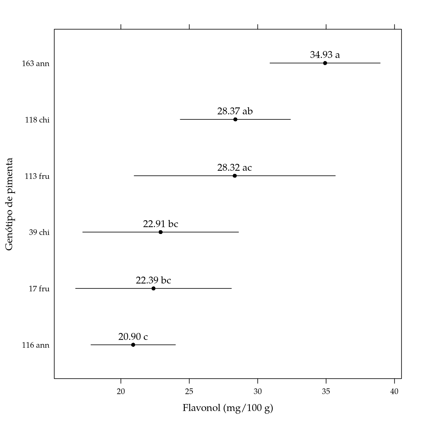
Antocianinas
# Exploratória.
xyplot(antoc ~ ldose | genab,
       data = dd) +
    layer(panel.smoother(x, y,
                         method = "lm",
                         form = y ~ poly(x, degree = 2), ...))
# Declara modelo fatorial com dose expresso por polinômio de grau 2.
m0 <- lm(antoc ~ genab * poly(ldose, degree = 2),
         data = dd)
anova(m0)
## Analysis of Variance Table
##
## Response: antoc
## Df Sum Sq Mean Sq F value Pr(>F)
## genab 5 833.10 166.619 25.9623 2.165e-10
## poly(ldose, degree = 2) 2 9.51 4.756 0.7411 0.4846
## genab:poly(ldose, degree = 2) 9 51.88 5.765 0.8982 0.5381
## Residuals 32 205.37 6.418
##
## genab ***
## poly(ldose, degree = 2)
## genab:poly(ldose, degree = 2)
## Residuals
## ---
## Signif. codes: 0 '***' 0.001 '**' 0.01 '*' 0.05 '.' 0.1 ' ' 1# par(mfrow = c(2, 2))
# plot(m0); layout(1)
# MASS::boxcox(m0)
# Declara o modelo reduzido contendo apenas o efeito de genótipo.
m1 <- update(m0, . ~ genab)
anova(m1, m0)## Analysis of Variance Table
##
## Model 1: antoc ~ genab
## Model 2: antoc ~ genab * poly(ldose, degree = 2)
## Res.Df RSS Df Sum of Sq F Pr(>F)
## 1 43 266.76
## 2 32 205.37 11 61.394 0.8697 0.5771# Comparações múltiplas entre médias de genótipos.
L <- LE_matrix(m1, effect = "genab")
rownames(L) <- attr(L, "grid")$genab
pred <- apmc(L, m1, "genab", test = "fdr")
arrange(pred, -fit)## genab fit lwr upr cld
## 1 163 ann 13.172333 11.583906 14.760761 a
## 2 39 chi 10.333667 8.087291 12.580043 ab
## 3 17 fru 9.646667 7.400291 11.893043 b
## 4 118 chi 5.907333 4.318906 7.495761 c
## 5 113 fru 4.773333 1.221501 8.325166 cd
## 6 116 ann 2.530000 1.311732 3.748268 d# Gráfico de segmentos.
segplot(reorder(genab, fit) ~ lwr + upr,
centers = fit,
data = pred,
cld = sprintf("%0.2f %s", pred$fit, pred$cld),
draw = FALSE,
xlab = "Antocianinas (mg/100 g)",
ylab = "Genótipo de pimenta") +
layer(panel.text(x = centers,
y = z,
labels = cld,
pos = 3))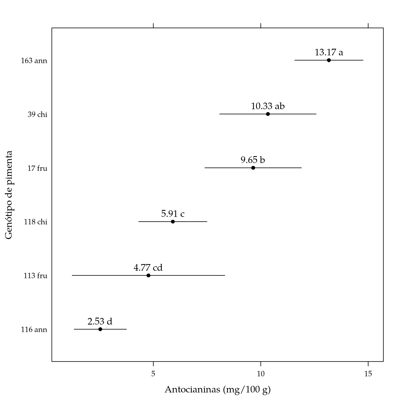
Informações da Sessão
## Atualizado em 11 de julho de 2019.
##
## R version 3.6.1 (2019-07-05)
## Platform: x86_64-pc-linux-gnu (64-bit)
## Running under: Ubuntu 18.04.2 LTS
##
## Matrix products: default
## BLAS:   /usr/lib/x86_64-linux-gnu/blas/libblas.so.3.7.1
## LAPACK: /usr/lib/x86_64-linux-gnu/lapack/liblapack.so.3.7.1
##
## locale:
##  [1] LC_CTYPE=pt_BR.UTF-8       LC_NUMERIC=C
##  [3] LC_TIME=pt_BR.UTF-8        LC_COLLATE=en_US.UTF-8
##  [5] LC_MONETARY=pt_BR.UTF-8    LC_MESSAGES=en_US.UTF-8
##  [7] LC_PAPER=pt_BR.UTF-8       LC_NAME=C
##  [9] LC_ADDRESS=C               LC_TELEPHONE=C
## [11] LC_MEASUREMENT=pt_BR.UTF-8 LC_IDENTIFICATION=C
##
## attached base packages:
## [1] stats     graphics  grDevices utils     datasets  methods
## [7] base
##
## other attached packages:
##  [1] candisc_0.8-0       heplots_1.3-5       car_3.0-3
##  [4] carData_3.0-2       multcomp_1.4-10     TH.data_1.0-10
##  [7] MASS_7.3-51.4       survival_2.44-1.1   mvtnorm_1.0-11
## [10] doBy_4.6-2          plyr_1.8.4          EACS_0.0-7
## [13] wzRfun_0.91         captioner_2.2.3     latticeExtra_0.6-28
## [16] RColorBrewer_1.1-2  lattice_0.20-38     knitr_1.23
##
## loaded via a namespace (and not attached):
##  [1] pkgload_1.0.2     splines_3.6.1     assertthat_0.2.1
##  [4] cellranger_1.1.0  yaml_2.2.0        remotes_2.1.0
##  [7] corrplot_0.84     sessioninfo_1.1.1 pillar_1.4.2
## [10] backports_1.1.4   glue_1.3.1        digest_0.6.20
## [13] sandwich_2.5-1    htmltools_0.3.6   Matrix_1.2-17
## [16] pkgconfig_2.0.2   devtools_2.1.0    haven_2.1.1
## [19] purrr_0.3.2       processx_3.4.0    openxlsx_4.1.0.1
## [22] rio_0.5.16        tibble_2.1.3      usethis_1.5.1
## [25] withr_2.1.2       cli_1.1.0         magrittr_1.5
## [28] crayon_1.3.4      readxl_1.3.1      memoise_1.1.0
## [31] evaluate_0.14     ps_1.3.0          fs_1.3.1
## [34] forcats_0.4.0     xml2_1.2.0        foreign_0.8-71
## [37] pkgbuild_1.0.3    tools_3.6.1       data.table_1.12.2
## [40] prettyunits_1.0.2 hms_0.5.0         stringr_1.4.0
## [43] zip_2.0.3         callr_3.3.0       compiler_3.6.1
## [46] pkgdown_1.3.0     rlang_0.4.0       grid_3.6.1
## [49] rstudioapi_0.10   rmarkdown_1.13    testthat_2.1.1
## [52] codetools_0.2-16  abind_1.4-5       roxygen2_6.1.1
## [55] curl_3.3          R6_2.4.0          zoo_1.8-6
## [58] dplyr_0.8.3       zeallot_0.1.0     commonmark_1.7
## [61] rprojroot_1.3-2   desc_1.2.0        stringi_1.4.3
## [64] Rcpp_1.0.1        vctrs_0.2.0       tidyselect_0.2.5
## [67] xfun_0.8