Cinza de cana em substrato de “terra de barranco” para produção de mudas de maracujazeiro
Milson E. Serafim & Walmes M. Zeviani
11 de julho de 2019
Source:vignettes/maracuja.Rmd
maracuja.RmdDefinições da sessão
#-----------------------------------------------------------------------
# Definições da sessão, pacotes a serem usados.

# Instruções para instalação do wzRfun em:
# browseURL("https://github.com/walmes/wzRfun")

pkg <- c("lattice", "latticeExtra", "grid", "gridExtra", "reshape",
         "plyr", "doBy", "multcomp", "MASS", "nlme", "wzRfun", "EACS")
sapply(pkg, library, character.only = TRUE, logical.return = TRUE)
## lattice latticeExtra grid gridExtra reshape plyr
## TRUE TRUE TRUE TRUE TRUE TRUE
## doBy multcomp MASS nlme wzRfun EACS
## TRUE TRUE TRUE TRUE TRUE TRUE#-----------------------------------------------------------------------
data(maracuja)
mara <- maracuja$cresc
str(mara)## 'data.frame': 1344 obs. of 7 variables:
## $ agreg: Factor w/ 2 levels "[0,2]","[4,10]": 2 2 2 2 2 2 2 2 2 2 ...
## $ fam : Factor w/ 2 levels "F29","F48": 1 1 1 1 1 1 1 1 1 1 ...
## $ cinz : num 0 0 0 0 0 0 1.5 1.5 1.5 1.5 ...
## $ bloc : Factor w/ 3 levels "1","2","3": 1 1 2 2 3 3 1 1 2 2 ...
## $ rept : int 1 2 1 2 1 2 1 2 1 2 ...
## $ data : Date, format: "2012-02-24" "2012-02-24" ...
## $ alt : num 6 6.5 4.5 4 4.5 4.5 8 7.2 6 7.4 ...mara <- transform(mara,
agreg = factor(agreg,
labels = c("0-2 mm", "4-10 mm")),
dias = as.numeric(data - min(data)))
str(mara)## 'data.frame': 1344 obs. of 8 variables:
## $ agreg: Factor w/ 2 levels "0-2 mm","4-10 mm": 2 2 2 2 2 2 2 2 2 2 ...
## $ fam : Factor w/ 2 levels "F29","F48": 1 1 1 1 1 1 1 1 1 1 ...
## $ cinz : num 0 0 0 0 0 0 1.5 1.5 1.5 1.5 ...
## $ bloc : Factor w/ 3 levels "1","2","3": 1 1 2 2 3 3 1 1 2 2 ...
## $ rept : int 1 2 1 2 1 2 1 2 1 2 ...
## $ data : Date, format: "2012-02-24" "2012-02-24" ...
## $ alt : num 6 6.5 4.5 4 4.5 4.5 8 7.2 6 7.4 ...
## $ dias : num 0 0 0 0 0 0 0 0 0 0 ...# ftable(xtabs(~bloc + fam + agreg + cinz + dias, data = mara))
# 3 bloc * 2 fam * 2 agreg * 7 cinz * 8 dias = 672 cells.
mara$id <- with(mara, interaction(bloc, fam, agreg, cinz, dias))
nlevels(mara$id)## [1] 672# Valores médios por parcela.
mara <- ddply(mara,
.(bloc, fam, agreg, cinz, dias),
summarise,
alt = mean(alt))
str(mara)## 'data.frame': 672 obs. of 6 variables:
## $ bloc : Factor w/ 3 levels "1","2","3": 1 1 1 1 1 1 1 1 1 1 ...
## $ fam : Factor w/ 2 levels "F29","F48": 1 1 1 1 1 1 1 1 1 1 ...
## $ agreg: Factor w/ 2 levels "0-2 mm","4-10 mm": 1 1 1 1 1 1 1 1 1 1 ...
## $ cinz : num 0 0 0 0 0 0 0 0 1.5 1.5 ...
## $ dias : num 0 6 14 21 28 35 42 47 0 6 ...
## $ alt : num 6.65 7.3 12.25 40.25 62.75 ...#-----------------------------------------------------------------------
# Ver.
xyplot(alt ~ dias | fam * agreg,
groups = cinz,
data = mara,
type = c("p", "a"))
#-----------------------------------------------------------------------
# Modelo para altura final.

m0 <- lm(alt ~ bloc + fam * agreg * cinz,
         data = subset(mara, dias == max(dias)))

# Resíduos.
# par(mfrow = c(2,2)); plot(m0); layout(1)

# Quadro de anova.
anova(m0)
## Analysis of Variance Table
##
## Response: alt
## Df Sum Sq Mean Sq F value Pr(>F)
## bloc 2 1475.6 737.79 4.8024 0.01094 *
## fam 1 184.5 184.53 1.2011 0.27665
## agreg 1 91.1 91.15 0.5933 0.44361
## cinz 1 5.8 5.82 0.0379 0.84626
## fam:agreg 1 0.1 0.07 0.0005 0.98250
## fam:cinz 1 539.5 539.53 3.5119 0.06488 .
## agreg:cinz 1 845.2 845.24 5.5018 0.02168 *
## fam:agreg:cinz 1 582.6 582.61 3.7923 0.05528 .
## Residuals 74 11368.7 153.63
## ---
## Signif. codes: 0 '***' 0.001 '**' 0.01 '*' 0.05 '.' 0.1 ' ' 1Crescimento das plantas via modelo não linear de efeitos aleatórios
#-----------------------------------------------------------------------
# Usando modelos não lineares mistos.

# Medidas repetidas nos indivíduos que são as parcelas.
mara$parcela <- with(mara,
                     interaction(bloc, fam, agreg, cinz, sep = "_"))
# nlevels(mara$parcela) # 3 * 2 * 2 * 7

marag <- groupedData(formula = alt ~ dias | parcela,
                     data = mara,
                     order = FALSE)
str(marag)
## Classes 'nfnGroupedData', 'nfGroupedData', 'groupedData' and 'data.frame': 672 obs. of 7 variables:
## $ bloc : Factor w/ 3 levels "1","2","3": 1 1 1 1 1 1 1 1 1 1 ...
## $ fam : Factor w/ 2 levels "F29","F48": 1 1 1 1 1 1 1 1 1 1 ...
## $ agreg : Factor w/ 2 levels "0-2 mm","4-10 mm": 1 1 1 1 1 1 1 1 1 1 ...
## $ cinz : num 0 0 0 0 0 0 0 0 1.5 1.5 ...
## $ dias : num 0 6 14 21 28 35 42 47 0 6 ...
## $ alt : num 6.65 7.3 12.25 40.25 62.75 ...
## $ parcela: Factor w/ 84 levels "1_F29_0-2 mm_0",..: 1 1 1 1 1 1 1 1 13 13 ...
## - attr(*, "formula")=Class 'formula' language alt ~ dias | parcela
## .. ..- attr(*, ".Environment")=<environment: R_GlobalEnv>
## - attr(*, "FUN")=function (x)
## - attr(*, "order.groups")= logi FALSE#-----------------------------------------------------------------------
# Modelo sem efeito dos fatores experimentais.
nn0 <- nlme(alt ~ SSlogis(dias, A, B, C),
fixed = A + B + C ~ 1,
random = A + B + C ~ 1,
data = marag,
start = list(fixed = c(148, 31, 6.8)))
# Quadro com as estimativas dos parâmetros.
summary(nn0)$tTable## Value Std.Error DF t-value p-value
## A 148.859024 0.9894452 586 150.44696 0.000000e+00
## B 31.428242 0.4685086 586 67.08146 3.732240e-277
## C 6.813377 0.1429614 586 47.65885 9.192973e-204VarCorr(nn0)## parcela = pdLogChol(list(A ~ 1,B ~ 1,C ~ 1))
## Variance StdDev Corr
## A 11.809208 3.436453 A B
## B 16.935643 4.115294 0.587
## C 1.085436 1.041843 -0.094 0.750
## Residual 24.159648 4.915246# intervals(nn0)
# plot(nn0)
# pairs(nn0)
# par(mfrow = c(1,3)); apply(ranef(nn0), 2, qqnorm); layout(1)
# Observações discrepantes.
outl <- which(abs(residuals(nn0, type = "pearson")) > 3)
outl## 1_F29_0-2 mm_3 1_F29_0-2 mm_3 1_F29_0-2 mm_48 1_F29_0-2 mm_48
## 23 24 54 55# Remoção.
marag <- marag[-outl, ]
#-----------------------------------------------------------------------
# O intercepto não é zero, não sei porque, mas incorporar no modelo.
# modelo: Int + A/(1 + exp(-(x - x0)/S)).
# modelo de efeitos aditivos, aleatório em A e B e modelagem da
# variância.
nn1 <- nlme(alt ~ int + A/(1 + exp(-(dias - d50)/S)),
fixed = list(int ~ 1,
A ~ bloc + fam + agreg + cinz,
d50 ~ bloc + fam + agreg + cinz,
S ~ bloc + fam + agreg + cinz),
random = A + d50 + S ~ 1,
data = marag,
start = list(
fixed = c(5,
120, 0, 0, 0, 0, 0,
30, 0, 0, 0, 0, 0,
4, 0, 0, 0, 0, 0)))
# Quadro de testes de Wald para termos de efeito fixo.
anova(nn1, type = "marginal")## numDF denDF F-value p-value
## int 1 566 407.7922 <.0001
## A.(Intercept) 1 566 2222.8190 <.0001
## A.bloc 2 566 2.1371 0.1190
## A.fam 1 566 0.1666 0.6833
## A.agreg 1 566 0.7575 0.3845
## A.cinz 1 566 0.0475 0.8276
## d50.(Intercept) 1 566 1339.3396 <.0001
## d50.bloc 2 566 4.0130 0.0186
## d50.fam 1 566 0.7058 0.4012
## d50.agreg 1 566 0.0999 0.7521
## d50.cinz 1 566 0.0461 0.8301
## S.(Intercept) 1 566 605.8578 <.0001
## S.bloc 2 566 0.9156 0.4009
## S.fam 1 566 1.0197 0.3130
## S.agreg 1 566 0.5373 0.4638
## S.cinz 1 566 0.6170 0.4325# summary(nn1)$tTable
VarCorr(nn1)## parcela = pdLogChol(list(A ~ 1,d50 ~ 1,S ~ 1))
## Variance StdDev Corr
## A.(Intercept) 95.9259512 9.7941795 A.(In) d50.(I
## d50.(Intercept) 8.7669259 2.9608995 -0.308
## S.(Intercept) 0.4800422 0.6928508 -0.436 0.338
## Residual 9.2030347 3.0336504# plot(nn1)
# par(mfrow = c(1,3)); apply(ranef(nn1), 2, qqnorm); layout(1)
# intervals(nn1)
# Pelo modelo acima ninguém interfere no crescimento da planta.
#-----------------------------------------------------------------------
# Modelo com interações.
nn2 <- nlme(alt ~ int + A/(1 + exp(-(dias - d50)/S)),
fixed = list(int ~ 1,
A ~ bloc + fam * agreg * cinz,
d50 ~ bloc + fam * agreg * cinz,
S ~ bloc + fam * agreg * cinz) ,
random = A + d50 + S ~ 1,
data = marag,
start = list(
fixed = c(5.2,
120, 0, 0, 0, 0, 0, 0, 0, 0, 0,
30, 0, 0, 0, 0, 0, 0, 0, 0, 0,
4, 0, 0, 0, 0, 0, 0, 0, 0, 0)))
anova(nn2, type = "marginal")## numDF denDF F-value p-value
## int 1 554 402.3897 <.0001
## A.(Intercept) 1 554 1535.2986 <.0001
## A.bloc 2 554 2.5664 0.0777
## A.fam 1 554 0.2935 0.5882
## A.agreg 1 554 4.5184 0.0340
## A.cinz 1 554 2.7408 0.0984
## A.fam:agreg 1 554 3.8955 0.0489
## A.fam:cinz 1 554 0.4822 0.4877
## A.agreg:cinz 1 554 13.2220 0.0003
## A.fam:agreg:cinz 1 554 6.0631 0.0141
## d50.(Intercept) 1 554 856.3358 <.0001
## d50.bloc 2 554 3.9352 0.0201
## d50.fam 1 554 1.3244 0.2503
## d50.agreg 1 554 0.0026 0.9590
## d50.cinz 1 554 0.3589 0.5494
## d50.fam:agreg 1 554 0.0004 0.9844
## d50.fam:cinz 1 554 0.8689 0.3517
## d50.agreg:cinz 1 554 0.0532 0.8176
## d50.fam:agreg:cinz 1 554 0.0103 0.9192
## S.(Intercept) 1 554 412.4307 <.0001
## S.bloc 2 554 0.9206 0.3989
## S.fam 1 554 0.0169 0.8967
## S.agreg 1 554 0.0324 0.8572
## S.cinz 1 554 0.4351 0.5098
## S.fam:agreg 1 554 0.4105 0.5220
## S.fam:cinz 1 554 0.0376 0.8462
## S.agreg:cinz 1 554 0.0763 0.7825
## S.fam:agreg:cinz 1 554 0.0665 0.7967# summary(nn2)$tTable
VarCorr(nn2)## parcela = pdLogChol(list(A ~ 1,d50 ~ 1,S ~ 1))
## Variance StdDev Corr
## A.(Intercept) 79.7499115 8.930281 A.(In) d50.(I
## d50.(Intercept) 8.5177705 2.918522 -0.282
## S.(Intercept) 0.4705919 0.685997 -0.427 0.342
## Residual 9.1424988 3.023657# plot(nn2)
# par(mfrow = c(1,3)); apply(ranef(nn2), 2, qqnorm); layout(1)
# intervals(nn2)
# pairs(nn2)
# Esse parece ser um bom modelo, existe interação tripla apenas para A,
# o resto não muda.
#-----------------------------------------------------------------------
# Modelo que é uma redução do nn2.
nn3 <- nlme(alt ~ int + A/(1 + exp(-(dias - d50)/S)),
fixed = list(int ~ 1,
A ~ bloc + fam * agreg * cinz,
d50 ~ bloc,
S ~ bloc) ,
random = A + d50 + S ~ 1,
data = marag,
start = list(
fixed = c(5.2,
120, 0, 0, 0, 0, 0, 0, 0, 0, 0,
30, 0, 0,
4, 0, 0)))
anova(nn3, type = "marginal")## numDF denDF F-value p-value
## int 1 568 412.3290 <.0001
## A.(Intercept) 1 568 1560.5222 <.0001
## A.bloc 2 568 2.7822 0.0627
## A.fam 1 568 0.5016 0.4791
## A.agreg 1 568 4.6332 0.0318
## A.cinz 1 568 2.9860 0.0845
## A.fam:agreg 1 568 4.0123 0.0456
## A.fam:cinz 1 568 0.7334 0.3922
## A.agreg:cinz 1 568 13.1341 0.0003
## A.fam:agreg:cinz 1 568 6.2785 0.0125
## d50.(Intercept) 1 568 2629.1886 <.0001
## d50.bloc 2 568 3.7369 0.0244
## S.(Intercept) 1 568 1189.7212 <.0001
## S.bloc 2 568 0.8326 0.4355anova(nn3, nn2) # Ótimo!!## Model df AIC BIC logLik Test L.Ratio p-value
## nn3 1 24 4077.136 4185.239 -2014.568
## nn2 2 38 4098.983 4270.146 -2011.492 1 vs 2 6.152922 0.9625summary(nn3)$tTable## Value Std.Error DF t-value p-value
## int 5.0500618 0.2486994 568 20.3058853 2.494136e-69
## A.(Intercept) 134.6840663 3.4094258 568 39.5034458 4.491832e-165
## A.bloc2 -1.3151716 2.7302320 568 -0.4817069 6.301997e-01
## A.bloc3 -6.2797696 2.7979816 568 -2.2443927 2.519135e-02
## A.famF48 2.9419669 4.1539590 568 0.7082321 4.790917e-01
## A.agreg4-10 mm 8.8981452 4.1338704 568 2.1524974 3.177875e-02
## A.cinz 0.2513645 0.1454649 568 1.7280072 8.453044e-02
## A.famF48:agreg4-10 mm -11.7083756 5.8451943 568 -2.0030772 4.564365e-02
## A.famF48:cinz -0.1692116 0.1975917 568 -0.8563702 3.921542e-01
## A.agreg4-10 mm:cinz -0.7410296 0.2044724 568 -3.6241049 3.159848e-04
## A.famF48:agreg4-10 mm:cinz 0.6993170 0.2790910 568 2.5056948 1.249973e-02
## d50.(Intercept) 30.0030415 0.5851328 568 51.2756144 2.803014e-215
## d50.bloc2 0.4303096 0.8260992 568 0.5208934 6.026440e-01
## d50.bloc3 2.1504465 0.8315168 568 2.5861731 9.952520e-03
## S.(Intercept) 5.6847067 0.1648107 568 34.4923359 1.897106e-141
## S.bloc2 -0.1758818 0.2261536 568 -0.7777098 4.370639e-01
## S.bloc3 0.1188585 0.2316284 568 0.5131432 6.080507e-01VarCorr(nn3)## parcela = pdLogChol(list(A ~ 1,d50 ~ 1,S ~ 1))
## Variance StdDev Corr
## A.(Intercept) 80.9886040 8.9993669 A.(In) d50.(I
## d50.(Intercept) 8.8801921 2.9799651 -0.273
## S.(Intercept) 0.4894687 0.6996204 -0.413 0.343
## Residual 9.1305216 3.0216753# plot(nn3)
# par(mfrow = c(1,3)); apply(ranef(nn3), 2, qqnorm); layout(1)
# intervals(nn3)
# pairs(nn3)
#-----------------------------------------------------------------------
# Fazendo a predição.
pred <- expand.grid(bloc = "1",
fam = levels(mara$fam),
agreg = levels(mara$agreg),
cinz = seq(0, 50, l = 2),
dias = seq(0, 60, l = 30))
pred$y <- predict(nn3, newdata = pred, level = 0)
xyplot(y ~ dias | fam * agreg,
groups = cinz,
data = pred,
type = c("l"))
# Largura da página da coluna da revista (8 cm = 3.150 pol) e da folha
# (17 cm = 6.690 pol).

colr <- c("white", "black")
colr <- colorRampPalette(colr, space = "rgb")

wireframe(y ~ dias + cinz|fam * agreg,
          data = pred,
          scales = list(arrows = FALSE),
          drape = TRUE,
          zlim = c(0, 155),
          zlab = list(expression(Altura ~ da ~ planta ~ (cm)),
                      rot = 90,
                      hjust = 0.5,
                      vjust = -0.2),
          xlab = list(expression(Dias),
                      vjust = 1,
                      rot = 30),
          ylab = list(expression(Cinza ~ (t ~ ha^{-1})),
                      vjust = 1,
                      rot = -40),
          strip = strip_combined,
          par.strip.text = list(lines = 0.6),
          par.settings = list(
              regions = list(col = colr(100)),
              layout.widths = list(xlab.axis.padding = 3)))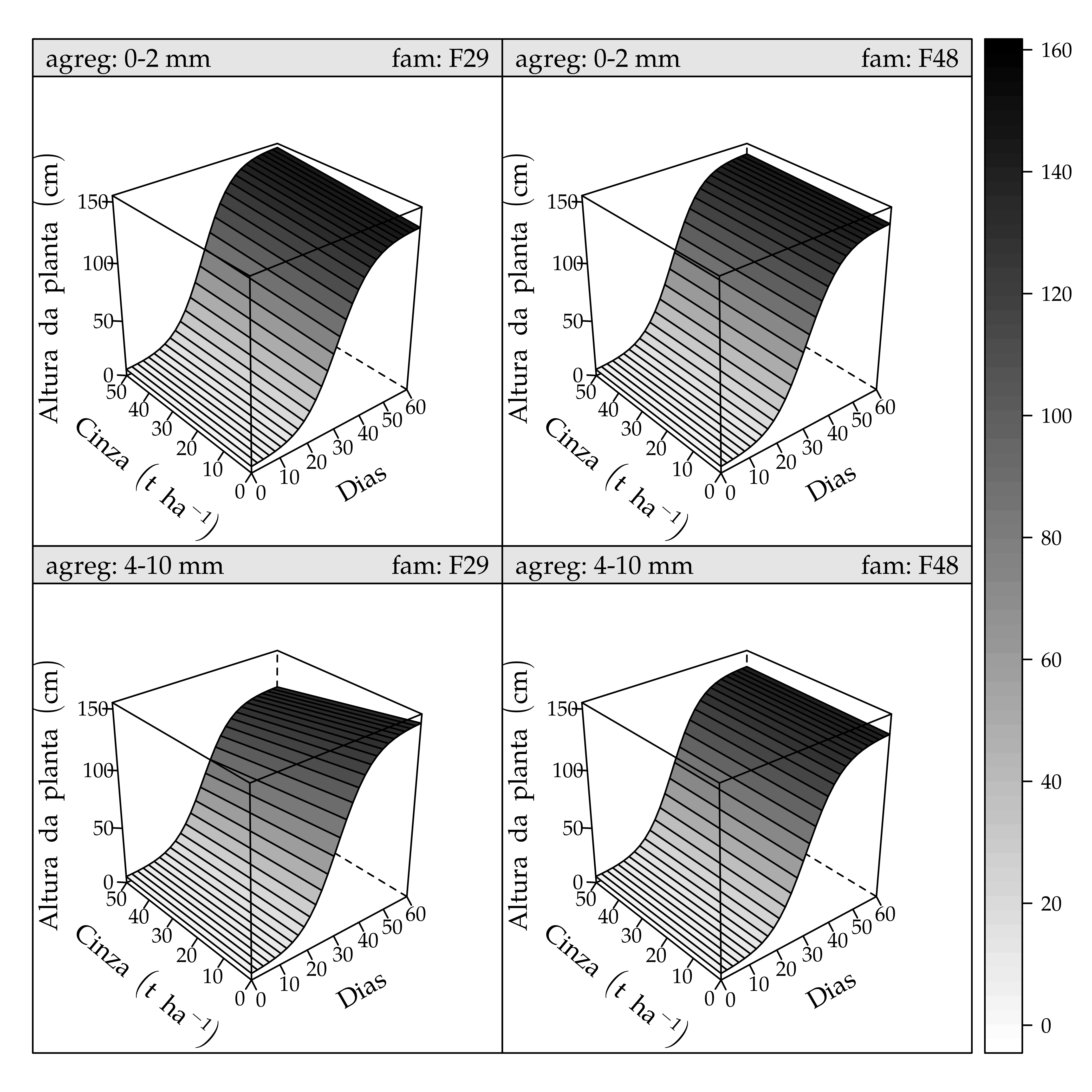
## [1] "fam"   "agreg"
## [1] "fam"   "agreg"
## [1] "fam"   "agreg"
## [1] "fam"   "agreg"
## [1] "fam"   "agreg"
## [1] "fam"   "agreg"
## [1] "fam"   "agreg"
## [1] "fam"   "agreg"
#-----------------------------------------------------------------------
# Estimativas pontuais das assíntotas.
summ <- summary(nn3)$tTable
summ[grep("cinz", rownames(summ)), ]## Value Std.Error DF t-value p-value
## A.cinz 0.2513645 0.1454649 568 1.7280072 0.0845304386
## A.famF48:cinz -0.1692116 0.1975917 568 -0.8563702 0.3921541819
## A.agreg4-10 mm:cinz -0.7410296 0.2044724 568 -3.6241049 0.0003159848
## A.famF48:agreg4-10 mm:cinz 0.6993170 0.2790910 568 2.5056948 0.0124997325coefs <- fixef(nn3)
vcovs <- vcov(nn3)
# names(coefs)
idA <- grep("^A\\.", names(coefs))
coefsA <- coefs[idA]
vcovsA <- vcovs[idA, idA]
# length(coefsA); length(coef(m0))
X0 <- LE_matrix(m0, effect = c("agreg", "fam"), at = list(cinz = 0))
b0 <- X0 %*% coefsA
v0 <- sqrt(diag(X0 %*% vcovsA %*% t(X0)))
ic0 <- sapply(1:4, function(i) b0[i] + c(-1, 0, 1) * 1.96 * v0[i])
ic0 <- t(ic0)
colnames(ic0) <- c("Lower", "Estimate", "Upper")
rownames(ic0) <- paste(c(outer(levels(mara$fam),
levels(mara$agreg),
paste)), "cinz 0")
X48 <- LE_matrix(m0, effect = c("agreg", "fam"), at = list(cinz = 48))
b48 <- X48 %*% coefsA
v48 <- sqrt(diag(X48 %*% vcovsA %*% t(X48)))
ic48 <- sapply(1:4, function(i) b48[i] + c(-1, 0, 1) * 1.96 * v48[i])
ic48 <- t(ic48)
colnames(ic48) <- c("Lower", "Estimate", "Upper")
rownames(ic48) <- paste(c(outer(levels(mara$fam),
levels(mara$agreg),
paste)), "cinz 48")
ics <- cbind(trat = c(rownames(ic0),
rownames(ic48)),
data.frame(rbind(ic0, ic48)))
p1 <-
segplot(reorder(trat, Estimate) ~ Lower + Upper,
data = ics,
draw.bands = FALSE,
centers = Estimate,
segments.fun = panel.arrows,
ends = "both",
angle = 90,
length = .05,
par.settings = simpleTheme(pch = 19, col = 1),
ylab = NULL,
xlab = expression(Ganho ~ em ~ altura ~ (cm)),
panel = function(x, y, z, ...) {
panel.abline(h = z, col = "grey", lty = "dashed")
panel.abline(v = 0, col = 1, lty = "dashed")
panel.segplot(x, y, z, ...)
})
# print(p1)
#-----------------------------------------------------------------------
# Mas o contraste é uma matriz menos a outra, então.
X <- X48 - X0
b <- X %*% coefsA
v <- X %*% vcovsA %*% t(X)
t <- b/sqrt(diag(v))
Z <- model.matrix(~fam * agreg,
expand.grid(fam = levels(mara$fam),
agreg = levels(mara$agreg)))
d <- coefs[grep("cinz", names(coefs))]
u <- vcovs[grep("cinz", names(coefs)),
grep("cinz", names(coefs))]
d <- c(Z %*% d)
u <- sqrt(diag(Z %*% u %*% t(Z)))
ic <- sapply(1:4, function(i) d[i] + c(-1, 0, 1) * 1.96 * u[i])
ic <- t(ic)
colnames(ic) <- c("Lower", "Estimate", "Upper")
rownames(ic) <- c(outer(levels(mara$fam),
levels(mara$agreg),
paste))
ic <- cbind(trat = rownames(ic), as.data.frame(ic))
p2 <- segplot(reorder(trat, Estimate) ~ Lower + Upper,
data = ic,
draw.bands = FALSE,
centers = Estimate,
segments.fun = panel.arrows,
ends = "both",
angle = 90,
length = .05,
par.settings = simpleTheme(pch = 19, col = 1),
ylab = NULL,
xlab = "Coeficiente de inclinação",
panel = function(x, y, z, ...) {
panel.abline(h = z, col = "grey", lty = "dashed")
panel.abline(v = 0, col = 1, lty = "dashed")
panel.segplot(x, y, z, ...)
})
# print(p2)plot(p1, split = c(1, 1, 1, 2), more = TRUE)
grid.text(label = "A", 0.025, 0.975)
plot(p2, split = c(1, 2, 1, 2), more = FALSE)
grid.text(label = "B", 0.025, 0.475)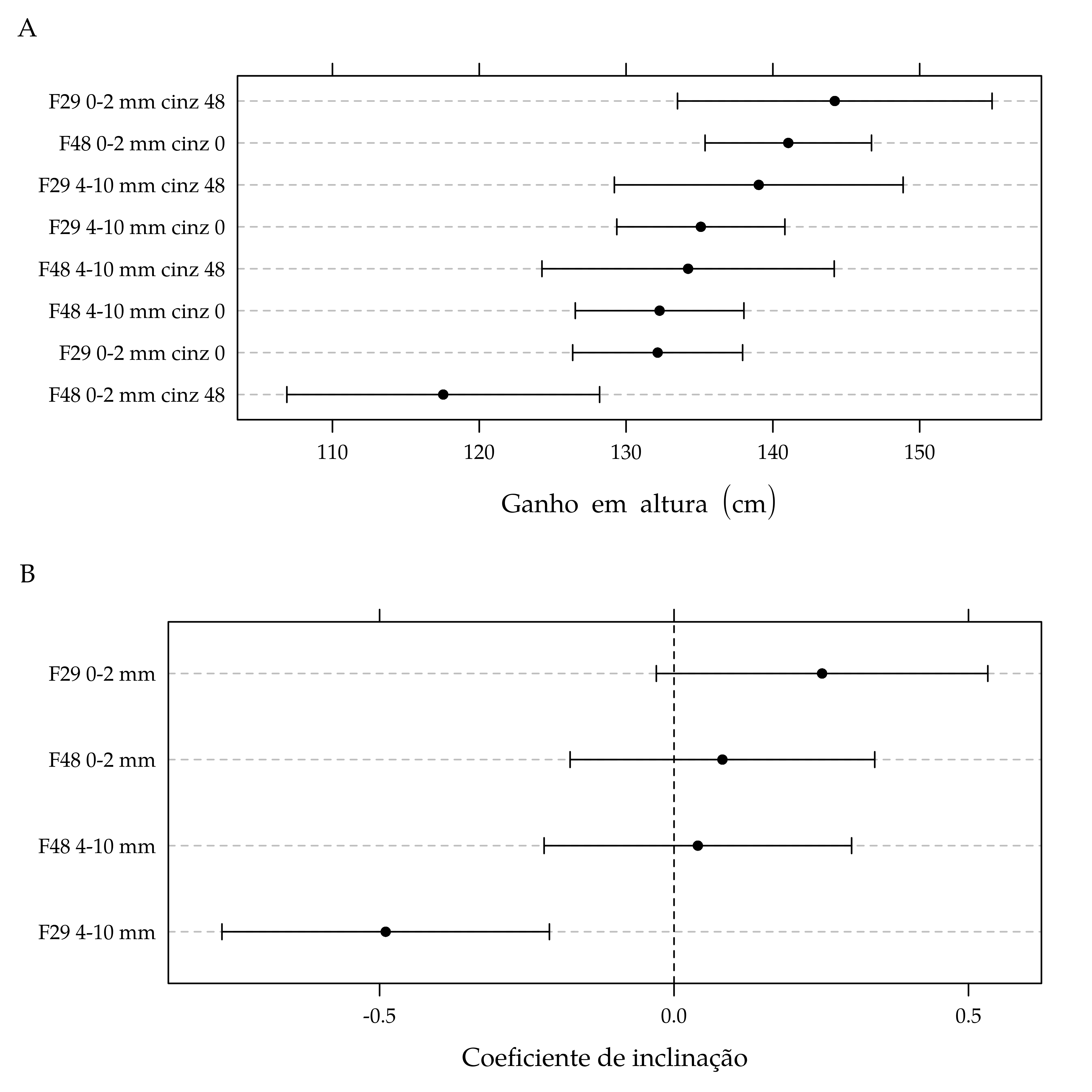
MSPA, MFPA, DS e CAV
#-----------------------------------------------------------------------
# Ler tabela de dados.

da <- maracuja$final
da <- transform(da,
                agreg = factor(agreg,
                               labels = c("0-2 mm", "4-10 mm")))
str(da)
## 'data.frame': 168 obs. of 9 variables:
## $ agreg: Factor w/ 2 levels "0-2 mm","4-10 mm": 2 2 2 2 2 2 2 2 2 2 ...
## $ fam : Factor w/ 2 levels "F29","F48": 1 1 1 1 1 1 1 1 1 1 ...
## $ cinz : num 0 0 0 0 0 0 1.5 1.5 1.5 1.5 ...
## $ bloc : Factor w/ 3 levels "1","2","3": 1 1 2 2 3 3 1 1 2 2 ...
## $ rept : int 1 2 1 2 1 2 1 2 1 2 ...
## $ mfpa : num 43.5 43.7 31.8 23.4 36.4 ...
## $ mspa : num 11.1 11.13 8.24 5.39 9.04 ...
## $ ds : num 1.24 1.25 1.23 1.23 1.27 1.18 1.27 1.28 1.01 1.19 ...
## $ cav : num 6470 7260 9446 9046 8468 ...## u
## [1,] 0.0 0 0.000000 -Inf
## [2,] 1.5 1 1.000000 0
## [3,] 3.0 2 1.414214 1
## [4,] 6.0 4 2.000000 2
## [5,] 12.0 8 2.828427 3
## [6,] 24.0 16 4.000000 4
## [7,] 48.0 32 5.656854 5# Doses de cinza em uma escala com distância mais regular entre níveis.
da$cin <- sqrt(da$cinz/1.5)
#-----------------------------------------------------------------------
# Ver.
combineLimits(
useOuterStrips(
xyplot(mfpa + mspa + ds + cav ~ cin | fam,
outer = TRUE,
groups = agreg,
data = da,
xlab = "Cinza (escala transformada)",
ylab = "Valor das variáveis resposta",
type = c("p", "smooth"),
auto.key = list(columns = 2,
title = "Classe de agregado",
cex.title = 1),
scales = list(y = "free"))))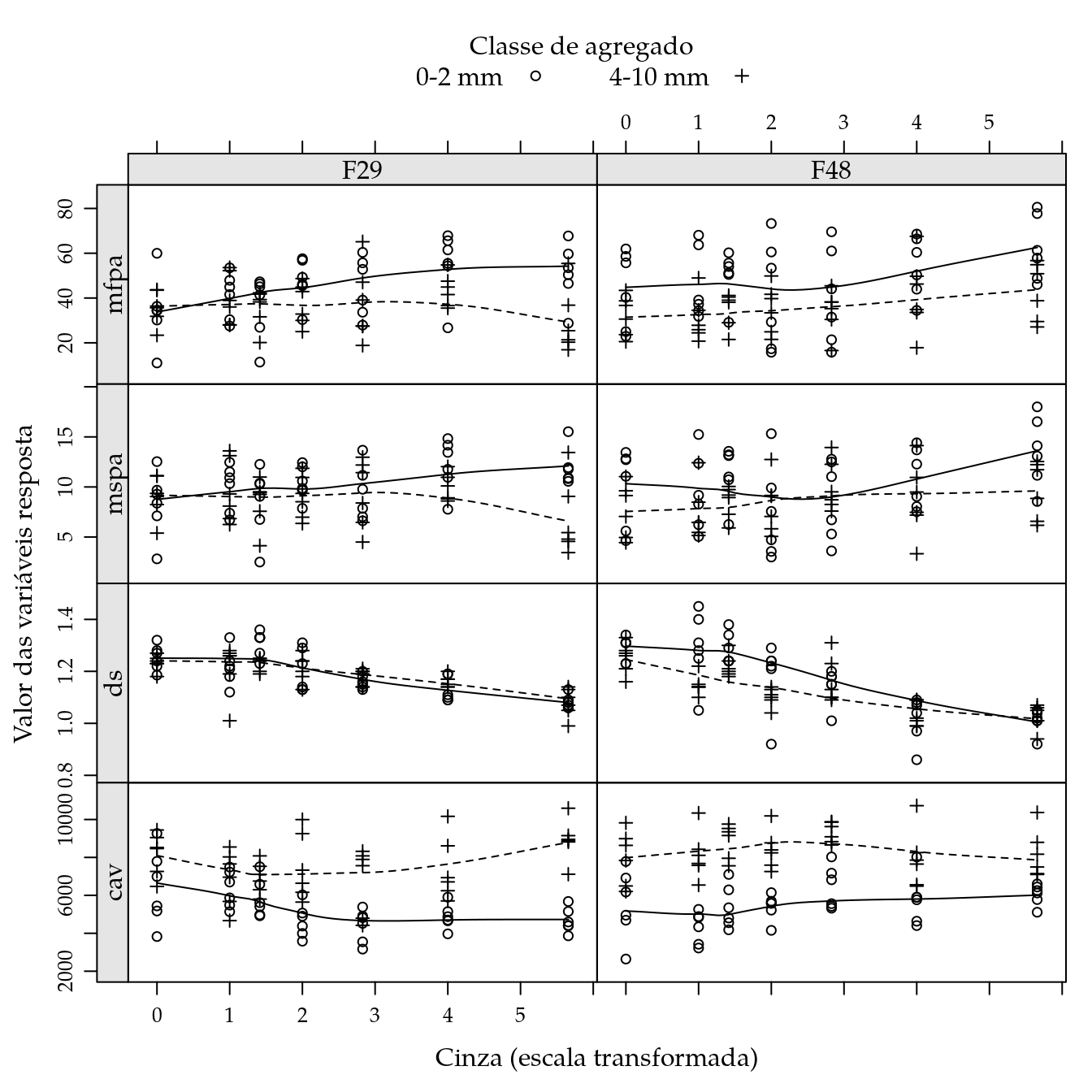
#-----------------------------------------------------------------------
# Especificação e ajuste dos modelos em batelada.

# Respostas.
resp <- c("mfpa", "mspa", "ds", "cav")

# Lista de formulas.
form0 <- lapply(paste(resp,
                      "~ bloc + fam * agreg * (cinz + I(cinz^2))"),
                as.formula)
names(form0) <- resp

# Ajustes.
m0 <- lapply(form0, lm, data = da)

#-----------------------------------------------------------------------
# Quadros de anova.

lapply(m0, anova)
## $mfpa
## Analysis of Variance Table
##
## Response: mfpa
## Df Sum Sq Mean Sq F value Pr(>F)
## bloc 2 2103.5 1051.8 6.5549 0.001853 **
## fam 1 88.7 88.7 0.5525 0.458424
## agreg 1 4129.9 4129.9 25.7388 1.111e-06 ***
## cinz 1 1848.3 1848.3 11.5191 0.000876 ***
## I(cinz^2) 1 426.3 426.3 2.6569 0.105148
## fam:agreg 1 257.8 257.8 1.6065 0.206896
## fam:cinz 1 431.2 431.2 2.6872 0.103198
## fam:I(cinz^2) 1 559.1 559.1 3.4847 0.063841 .
## agreg:cinz 1 839.9 839.9 5.2348 0.023500 *
## agreg:I(cinz^2) 1 26.5 26.5 0.1654 0.684839
## fam:agreg:cinz 1 252.3 252.3 1.5726 0.211733
## fam:agreg:I(cinz^2) 1 122.8 122.8 0.7652 0.383074
## Residuals 154 24710.0 160.5
## ---
## Signif. codes: 0 '***' 0.001 '**' 0.01 '*' 0.05 '.' 0.1 ' ' 1
##
## $mspa
## Analysis of Variance Table
##
## Response: mspa
## Df Sum Sq Mean Sq F value Pr(>F)
## bloc 2 86.24 43.121 5.2662 0.006134 **
## fam 1 0.32 0.315 0.0385 0.844648
## agreg 1 80.26 80.261 9.8020 0.002086 **
## cinz 1 61.76 61.758 7.5423 0.006745 **
## I(cinz^2) 1 4.97 4.970 0.6069 0.437143
## fam:agreg 1 1.24 1.245 0.1520 0.697172
## fam:cinz 1 20.51 20.512 2.5051 0.115529
## fam:I(cinz^2) 1 21.27 21.272 2.5979 0.109053
## agreg:cinz 1 63.03 63.027 7.6973 0.006215 **
## agreg:I(cinz^2) 1 13.61 13.609 1.6620 0.199267
## fam:agreg:cinz 1 11.24 11.240 1.3728 0.243147
## fam:agreg:I(cinz^2) 1 7.39 7.387 0.9021 0.343697
## Residuals 154 1260.98 8.188
## ---
## Signif. codes: 0 '***' 0.001 '**' 0.01 '*' 0.05 '.' 0.1 ' ' 1
##
## $ds
## Analysis of Variance Table
##
## Response: ds
## Df Sum Sq Mean Sq F value Pr(>F)
## bloc 2 0.04405 0.02203 5.0632 0.0074192 **
## fam 1 0.05306 0.05306 12.1962 0.0006252 ***
## agreg 1 0.02394 0.02394 5.5037 0.0202505 *
## cinz 1 0.81520 0.81520 187.3804 < 2.2e-16 ***
## I(cinz^2) 1 0.08952 0.08952 20.5770 1.146e-05 ***
## fam:agreg 1 0.01259 0.01259 2.8940 0.0909284 .
## fam:cinz 1 0.03576 0.03576 8.2192 0.0047257 **
## fam:I(cinz^2) 1 0.03236 0.03236 7.4382 0.0071268 **
## agreg:cinz 1 0.02580 0.02580 5.9314 0.0160155 *
## agreg:I(cinz^2) 1 0.01699 0.01699 3.9060 0.0499013 *
## fam:agreg:cinz 1 0.00661 0.00661 1.5188 0.2196819
## fam:agreg:I(cinz^2) 1 0.00008 0.00008 0.0187 0.8914281
## Residuals 154 0.66998 0.00435
## ---
## Signif. codes: 0 '***' 0.001 '**' 0.01 '*' 0.05 '.' 0.1 ' ' 1
##
## $cav
## Analysis of Variance Table
##
## Response: cav
## Df Sum Sq Mean Sq F value Pr(>F)
## bloc 2 4704295 2352148 1.5448 0.2166456
## fam 1 12968149 12968149 8.5169 0.0040462 **
## agreg 1 270606640 270606640 177.7222 < 2.2e-16 ***
## cinz 1 550533 550533 0.3616 0.5485225
## I(cinz^2) 1 2360352 2360352 1.5502 0.2150012
## fam:agreg 1 4240215 4240215 2.7848 0.0971955 .
## fam:cinz 1 581539 581539 0.3819 0.5374858
## fam:I(cinz^2) 1 14011881 14011881 9.2024 0.0028376 **
## agreg:cinz 1 2821636 2821636 1.8531 0.1754091
## agreg:I(cinz^2) 1 13641 13641 0.0090 0.9247148
## fam:agreg:cinz 1 19103685 19103685 12.5464 0.0005256 ***
## fam:agreg:I(cinz^2) 1 291877 291877 0.1917 0.6621261
## Residuals 154 234486288 1522638
## ---
## Signif. codes: 0 '***' 0.001 '**' 0.01 '*' 0.05 '.' 0.1 ' ' 1#-----------------------------------------------------------------------
# Quadro de estimativas dos efeitos.
lapply(m0, summary)## $mfpa
##
## Call:
## FUN(formula = X[[i]], data = ..1)
##
## Residuals:
## Min 1Q Median 3Q Max
## -33.074 -8.108 1.068 7.509 32.862
##
## Coefficients:
## Estimate Std. Error t value Pr(>|t|)
## (Intercept) 39.947583 3.468766 11.516 < 2e-16 ***
## bloc2 -2.623214 2.393848 -1.096 0.274871
## bloc3 -8.465893 2.393848 -3.537 0.000536 ***
## famF48 8.487977 4.499371 1.886 0.061113 .
## agreg4-10 mm -0.716554 4.499371 -0.159 0.873676
## cinz 1.212067 0.464685 2.608 0.009993 **
## I(cinz^2) -0.018792 0.009479 -1.982 0.049212 *
## famF48:agreg4-10 mm -12.400527 6.363071 -1.949 0.053133 .
## famF48:cinz -1.182186 0.657164 -1.799 0.073989 .
## famF48:I(cinz^2) 0.025987 0.013406 1.939 0.054389 .
## agreg4-10 mm:cinz -0.642157 0.657164 -0.977 0.330020
## agreg4-10 mm:I(cinz^2) 0.004437 0.013406 0.331 0.741092
## famF48:agreg4-10 mm:cinz 1.090510 0.929370 1.173 0.242452
## famF48:agreg4-10 mm:I(cinz^2) -0.016584 0.018958 -0.875 0.383074
## ---
## Signif. codes: 0 '***' 0.001 '**' 0.01 '*' 0.05 '.' 0.1 ' ' 1
##
## Residual standard error: 12.67 on 154 degrees of freedom
## Multiple R-squared: 0.3097, Adjusted R-squared: 0.2514
## F-statistic: 5.315 on 13 and 154 DF, p-value: 7.802e-08
##
##
## $mspa
##
## Call:
## FUN(formula = X[[i]], data = ..1)
##
## Residuals:
## Min 1Q Median 3Q Max
## -7.3162 -1.8967 0.2143 2.0662 6.9304
##
## Coefficients:
## Estimate Std. Error t value Pr(>|t|)
## (Intercept) 9.3129949 0.7835985 11.885 < 2e-16 ***
## bloc2 -0.2450000 0.5407732 -0.453 0.65115
## bloc3 -1.6275000 0.5407732 -3.010 0.00306 **
## famF48 1.0284923 1.0164134 1.012 0.31318
## agreg4-10 mm 0.1132211 1.0164134 0.111 0.91145
## cinz 0.1743295 0.1049729 1.661 0.09881 .
## I(cinz^2) -0.0021965 0.0021414 -1.026 0.30662
## famF48:agreg4-10 mm -2.0292102 1.4374256 -1.412 0.16006
## famF48:cinz -0.2481261 0.1484541 -1.671 0.09667 .
## famF48:I(cinz^2) 0.0054853 0.0030283 1.811 0.07204 .
## agreg4-10 mm:cinz -0.0744156 0.1484541 -0.501 0.61690
## agreg4-10 mm:I(cinz^2) -0.0007267 0.0030283 -0.240 0.81067
## famF48:agreg4-10 mm:cinz 0.2570117 0.2099458 1.224 0.22275
## famF48:agreg4-10 mm:I(cinz^2) -0.0040678 0.0042827 -0.950 0.34370
## ---
## Signif. codes: 0 '***' 0.001 '**' 0.01 '*' 0.05 '.' 0.1 ' ' 1
##
## Residual standard error: 2.862 on 154 degrees of freedom
## Multiple R-squared: 0.2277, Adjusted R-squared: 0.1625
## F-statistic: 3.493 on 13 and 154 DF, p-value: 8.922e-05
##
##
## $ds
##
## Call:
## FUN(formula = X[[i]], data = ..1)
##
## Residuals:
## Min 1Q Median 3Q Max
## -0.271875 -0.030538 0.003811 0.033212 0.179064
##
## Coefficients:
## Estimate Std. Error t value Pr(>|t|)
## (Intercept) 1.264e+00 1.806e-02 69.958 < 2e-16 ***
## bloc2 -2.099e-02 1.246e-02 -1.684 0.09417 .
## bloc3 1.865e-02 1.246e-02 1.496 0.13666
## famF48 4.518e-02 2.343e-02 1.929 0.05562 .
## agreg4-10 mm -3.503e-02 2.343e-02 -1.495 0.13695
## cinz -8.080e-03 2.420e-03 -3.339 0.00105 **
## I(cinz^2) 9.004e-05 4.936e-05 1.824 0.07005 .
## famF48:agreg4-10 mm -5.847e-02 3.313e-02 -1.765 0.07960 .
## famF48:cinz -9.292e-03 3.422e-03 -2.715 0.00738 **
## famF48:I(cinz^2) 1.414e-04 6.980e-05 2.025 0.04458 *
## agreg4-10 mm:cinz 5.060e-03 3.422e-03 1.479 0.14130
## agreg4-10 mm:I(cinz^2) -9.080e-05 6.980e-05 -1.301 0.19527
## famF48:agreg4-10 mm:cinz 2.205e-03 4.839e-03 0.456 0.64933
## famF48:agreg4-10 mm:I(cinz^2) -1.350e-05 9.872e-05 -0.137 0.89143
## ---
## Signif. codes: 0 '***' 0.001 '**' 0.01 '*' 0.05 '.' 0.1 ' ' 1
##
## Residual standard error: 0.06596 on 154 degrees of freedom
## Multiple R-squared: 0.6331, Adjusted R-squared: 0.6021
## F-statistic: 20.44 on 13 and 154 DF, p-value: < 2.2e-16
##
##
## $cav
##
## Call:
## FUN(formula = X[[i]], data = ..1)
##
## Residuals:
## Min 1Q Median 3Q Max
## -2658.0 -767.1 -123.3 800.8 3245.6
##
## Coefficients:
## Estimate Std. Error t value Pr(>|t|)
## (Intercept) 6018.4385 337.9074 17.811 < 2e-16 ***
## bloc2 -10.1964 233.1951 -0.044 0.96518
## bloc3 349.7679 233.1951 1.500 0.13569
## famF48 -1070.2391 438.3031 -2.442 0.01575 *
## agreg4-10 mm 1370.2799 438.3031 3.126 0.00212 **
## cinz -130.1812 45.2670 -2.876 0.00460 **
## I(cinz^2) 2.1339 0.9234 2.311 0.02217 *
## famF48:agreg4-10 mm 1934.0225 619.8542 3.120 0.00216 **
## famF48:cinz 201.0797 64.0171 3.141 0.00202 **
## famF48:I(cinz^2) -3.2055 1.3059 -2.455 0.01522 *
## agreg4-10 mm:cinz 73.2835 64.0171 1.145 0.25409
## agreg4-10 mm:I(cinz^2) -0.3169 1.3059 -0.243 0.80859
## famF48:agreg4-10 mm:cinz -122.4676 90.5339 -1.353 0.17813
## famF48:agreg4-10 mm:I(cinz^2) 0.8086 1.8468 0.438 0.66213
## ---
## Signif. codes: 0 '***' 0.001 '**' 0.01 '*' 0.05 '.' 0.1 ' ' 1
##
## Residual standard error: 1234 on 154 degrees of freedom
## Multiple R-squared: 0.5863, Adjusted R-squared: 0.5513
## F-statistic: 16.79 on 13 and 154 DF, p-value: < 2.2e-16#-----------------------------------------------------------------------
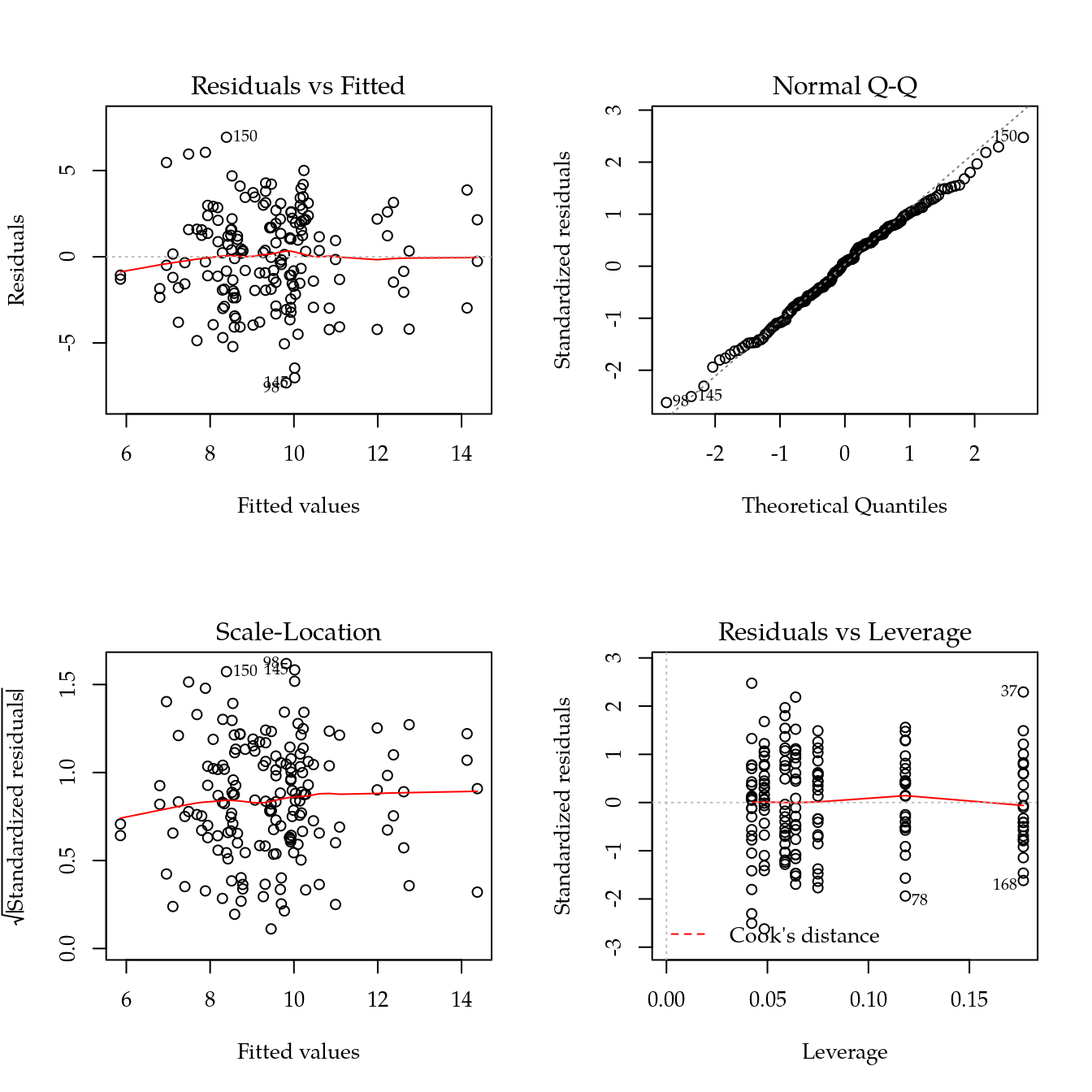
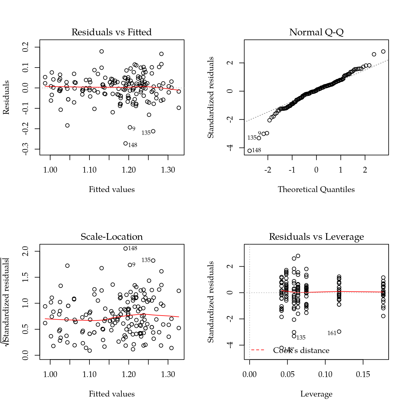
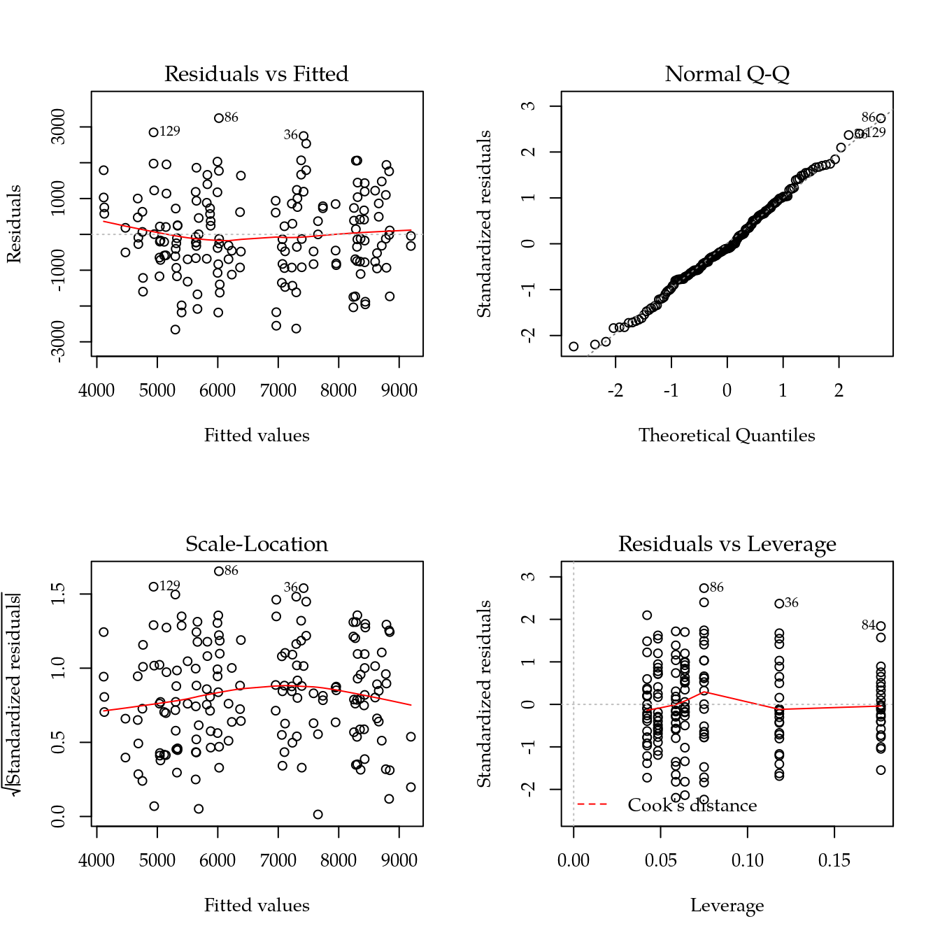
# Avaliação dos pressupostos.
par(mfrow = c(2,2)); plot(m0[["mfpa"]]); layout(1) ## ok!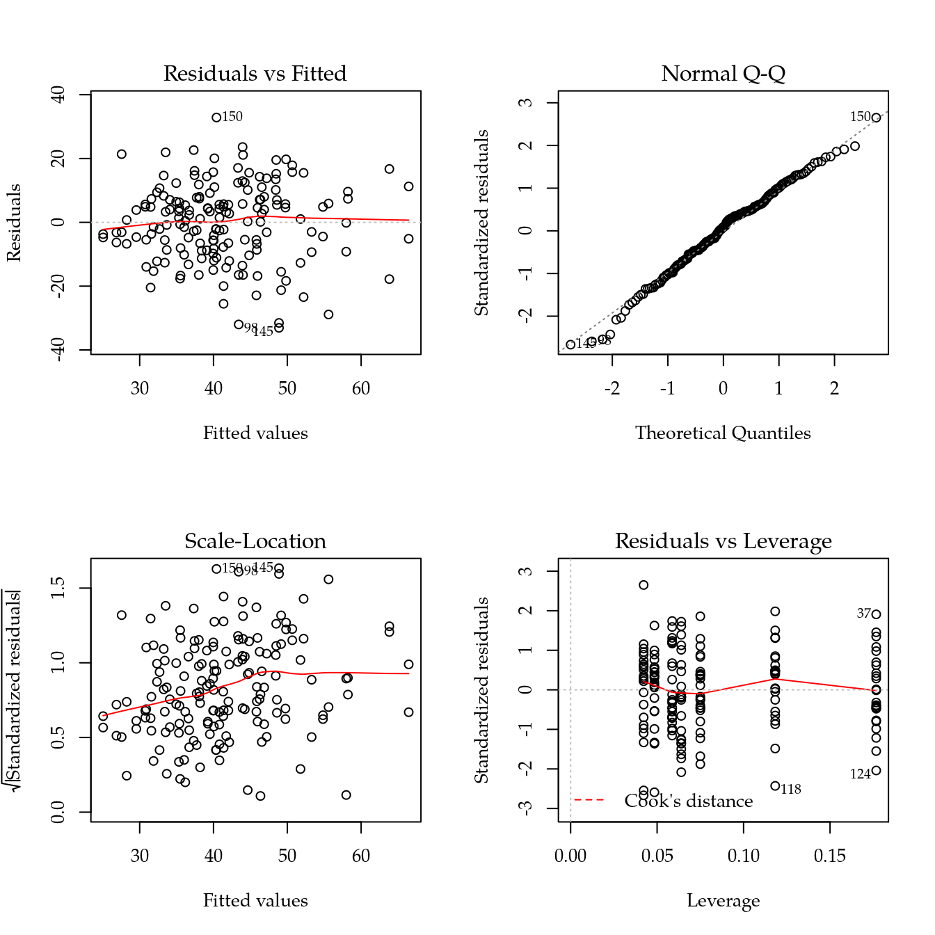
#-----------------------------------------------------------------------
# Modelos após abandono de termos não significativos.

form1 <- list(
    mfpa = mfpa ~ bloc + agreg * cinz,
    mspa = mspa ~ bloc + agreg * cinz,
    ds = ds ~ bloc + (fam + agreg + cinz)^3 + (fam + agreg) * I(cinz^2),
    cav = cav ~ bloc + fam * agreg * (cinz + I(cinz^2)))

m1 <- lapply(form1, lm, data = da, contrast = list(bloc = contr.sum))
lapply(m1, anova)
## $mfpa
## Analysis of Variance Table
##
## Response: mfpa
## Df Sum Sq Mean Sq F value Pr(>F)
## bloc 2 2103.5 1051.8 6.3401 0.002234 **
## agreg 1 4129.9 4129.9 24.8950 1.548e-06 ***
## cinz 1 1848.3 1848.3 11.1414 0.001047 **
## agreg:cinz 1 839.9 839.9 5.0632 0.025786 *
## Residuals 162 26874.6 165.9
## ---
## Signif. codes: 0 '***' 0.001 '**' 0.01 '*' 0.05 '.' 0.1 ' ' 1
##
## $mspa
## Analysis of Variance Table
##
## Response: mspa
## Df Sum Sq Mean Sq F value Pr(>F)
## bloc 2 86.24 43.121 5.2072 0.006431 **
## agreg 1 80.26 80.261 9.6921 0.002188 **
## cinz 1 61.76 61.758 7.4577 0.007016 **
## agreg:cinz 1 63.03 63.027 7.6110 0.006469 **
## Residuals 162 1341.53 8.281
## ---
## Signif. codes: 0 '***' 0.001 '**' 0.01 '*' 0.05 '.' 0.1 ' ' 1
##
## $ds
## Analysis of Variance Table
##
## Response: ds
## Df Sum Sq Mean Sq F value Pr(>F)
## bloc 2 0.04405 0.02203 5.0955 0.0071909 **
## fam 1 0.05306 0.05306 12.2739 0.0006005 ***
## agreg 1 0.02394 0.02394 5.5388 0.0198546 *
## cinz 1 0.81520 0.81520 188.5742 < 2.2e-16 ***
## I(cinz^2) 1 0.08952 0.08952 20.7081 1.074e-05 ***
## fam:agreg 1 0.01259 0.01259 2.9124 0.0899018 .
## fam:cinz 1 0.03576 0.03576 8.2716 0.0045943 **
## agreg:cinz 1 0.02580 0.02580 5.9691 0.0156812 *
## fam:I(cinz^2) 1 0.03236 0.03236 7.4856 0.0069454 **
## agreg:I(cinz^2) 1 0.01699 0.01699 3.9308 0.0491754 *
## fam:agreg:cinz 1 0.00661 0.00661 1.5285 0.2182139
## Residuals 155 0.67006 0.00432
## ---
## Signif. codes: 0 '***' 0.001 '**' 0.01 '*' 0.05 '.' 0.1 ' ' 1
##
## $cav
## Analysis of Variance Table
##
## Response: cav
## Df Sum Sq Mean Sq F value Pr(>F)
## bloc 2 4704295 2352148 1.5448 0.2166456
## fam 1 12968149 12968149 8.5169 0.0040462 **
## agreg 1 270606640 270606640 177.7222 < 2.2e-16 ***
## cinz 1 550533 550533 0.3616 0.5485225
## I(cinz^2) 1 2360352 2360352 1.5502 0.2150012
## fam:agreg 1 4240215 4240215 2.7848 0.0971955 .
## fam:cinz 1 581539 581539 0.3819 0.5374858
## fam:I(cinz^2) 1 14011881 14011881 9.2024 0.0028376 **
## agreg:cinz 1 2821636 2821636 1.8531 0.1754091
## agreg:I(cinz^2) 1 13641 13641 0.0090 0.9247148
## fam:agreg:cinz 1 19103685 19103685 12.5464 0.0005256 ***
## fam:agreg:I(cinz^2) 1 291877 291877 0.1917 0.6621261
## Residuals 154 234486288 1522638
## ---
## Signif. codes: 0 '***' 0.001 '**' 0.01 '*' 0.05 '.' 0.1 ' ' 1# Anova entre modelos sequenciais.
sapply(names(m1),
simplify = FALSE,
function(i) {
anova(m0[[i]], m1[[i]])
})## $mfpa
## Analysis of Variance Table
##
## Model 1: mfpa ~ bloc + fam * agreg * (cinz + I(cinz^2))
## Model 2: mfpa ~ bloc + agreg * cinz
## Res.Df RSS Df Sum of Sq F Pr(>F)
## 1 154 24710
## 2 162 26875 -8 -2164.7 1.6864 0.1058
##
## $mspa
## Analysis of Variance Table
##
## Model 1: mspa ~ bloc + fam * agreg * (cinz + I(cinz^2))
## Model 2: mspa ~ bloc + agreg * cinz
## Res.Df RSS Df Sum of Sq F Pr(>F)
## 1 154 1261.0
## 2 162 1341.5 -8 -80.55 1.2297 0.2852
##
## $ds
## Analysis of Variance Table
##
## Model 1: ds ~ bloc + fam * agreg * (cinz + I(cinz^2))
## Model 2: ds ~ bloc + (fam + agreg + cinz)^3 + (fam + agreg) * I(cinz^2)
## Res.Df RSS Df Sum of Sq F Pr(>F)
## 1 154 0.66998
## 2 155 0.67006 -1 -8.1325e-05 0.0187 0.8914
##
## $cav
## Analysis of Variance Table
##
## Model 1: cav ~ bloc + fam * agreg * (cinz + I(cinz^2))
## Model 2: cav ~ bloc + fam * agreg * (cinz + I(cinz^2))
## Res.Df RSS Df Sum of Sq F Pr(>F)
## 1 154 234486288
## 2 154 234486288 0 1.7881e-07#-----------------------------------------------------------------------
# Valores preditos.
gridlist <- list(bloc = "1",
fam = levels(da$fam),
agreg = levels(da$agreg),
cin = seq(0, 6, l = 100),
cinz = seq(0, 50, l = 100))
m1 <- lapply(m1,
function(i) {
predvars <- attr(terms(i), "term.labels")
pred <- do.call(
expand.grid,
gridlist[predvars[!sapply(gridlist[predvars],
is.null)]])
i$newdata <- pred
return(i)
})
mypredict <- function(m) {
cbind(m$newdata,
predict(m,
newdata = m$newdata,
interval = "confidence") -
coef(m)["bloc1"])
}
all.pred <- lapply(m1, mypredict)
# str(all.pred)
# lapply(all.pred, names)#-----------------------------------------------------------------------
# Gráficos.
xlab <- expression("Cinza" ~ (t ~ ha^{-1}))
ylab <- list(expression("Massa fresca de parte aérea" ~ (g)),
expression("Massa seca de parte aérea" ~ (g)),
expression("Densidade do solo" ~ (Mg ~ t^{-1})),
expression("Água consumida no ciclo" ~ (mL)))
names(ylab) <- names(m1)
l <- levels(da$agreg)
n <- nlevels(da$agreg)
key <- list(columns = 2,
title = "Classe de agregado (mm)",
cex.title = 1.1,
type = "o",
divide = 1,
text = list(l),
lines = list(
pch = trellis.par.get()$superpose.symbol$pch[1:n],
lty = trellis.par.get()$superpose.line$lty[1:n]))
scales <- list(alternating = 1)
#-----------------------------------------------------------------------
# MFPA.
p1 <- xyplot(mfpa ~ cinz,
groups = agreg,
data = da,
ylab = ylab[["mfpa"]],
xlab = xlab,
strip = strip.custom(bg = "gray90"),
key = key,
scales = scales) +
as.layer(with(all.pred[["mfpa"]],
xyplot(fit ~ cinz,
groups = agreg,
type = "l",
ly = lwr,
uy = upr,
cty = "bands",
fill = 1,
alpha = 0.2,
prepanel = prepanel.cbH,
panel = panel.superpose,
panel.groups = panel.cbH)))
#-----------------------------------------------------------------------
# MSPA.
p2 <- xyplot(mspa ~ cinz,
groups = agreg,
data = da,
ylab = ylab[["mspa"]],
xlab = xlab,
strip = strip.custom(bg = "gray90"),
key = key,
scales = scales) +
as.layer(with(all.pred[["mspa"]],
xyplot(fit ~ cinz,
groups = agreg,
type = "l",
ly = lwr,
uy = upr,
cty = "bands",
fill = 1,
alpha = 0.2,
prepanel = prepanel.cbH,
panel = panel.superpose,
panel.groups = panel.cbH)))
#-----------------------------------------------------------------------
# DS.
p3 <- xyplot(ds ~ cinz | fam,
groups = agreg,
data = da,
layout = c(NA, 1),
ylab = ylab[["ds"]],
xlab = NULL,
strip = strip.custom(bg = "gray90"),
key = key,
scales = scales) +
as.layer(with(all.pred[["ds"]],
xyplot(fit ~ cinz | fam,
groups = agreg,
type = "l",
ly = lwr,
uy = upr,
cty = "bands",
fill = 1,
alpha = 0.2,
prepanel = prepanel.cbH,
panel = panel.superpose,
panel.groups = panel.cbH)))
#-----------------------------------------------------------------------
# CAV.
p4 <- xyplot(cav ~ cinz | fam,
groups = agreg,
data = da,
layout = c(NA, 1),
ylab = ylab[["cav"]],
xlab = xlab,
strip = strip.custom(bg = "gray90"),
scales = scales) +
as.layer(with(all.pred[["cav"]],
xyplot(fit ~ cinz | fam,
groups = agreg,
type = "l",
ly = lwr,
uy = upr,
cty = "bands",
fill = 1,
alpha = 0.2,
prepanel = prepanel.cbH,
panel = panel.superpose,
panel.groups = panel.cbH)))Informações da Sessão
## Atualizado em 11 de julho de 2019.
##
## R version 3.6.1 (2019-07-05)
## Platform: x86_64-pc-linux-gnu (64-bit)
## Running under: Ubuntu 18.04.2 LTS
##
## Matrix products: default
## BLAS:   /usr/lib/x86_64-linux-gnu/blas/libblas.so.3.7.1
## LAPACK: /usr/lib/x86_64-linux-gnu/lapack/liblapack.so.3.7.1
##
## locale:
##  [1] LC_CTYPE=pt_BR.UTF-8       LC_NUMERIC=C
##  [3] LC_TIME=pt_BR.UTF-8        LC_COLLATE=en_US.UTF-8
##  [5] LC_MONETARY=pt_BR.UTF-8    LC_MESSAGES=en_US.UTF-8
##  [7] LC_PAPER=pt_BR.UTF-8       LC_NAME=C
##  [9] LC_ADDRESS=C               LC_TELEPHONE=C
## [11] LC_MEASUREMENT=pt_BR.UTF-8 LC_IDENTIFICATION=C
##
## attached base packages:
## [1] grid      stats     graphics  grDevices utils     datasets  methods
## [8] base
##
## other attached packages:
##  [1] nlme_3.1-140        multcomp_1.4-10     TH.data_1.0-10
##  [4] MASS_7.3-51.4       survival_2.44-1.1   mvtnorm_1.0-11
##  [7] doBy_4.6-2          plyr_1.8.4          reshape_0.8.8
## [10] gridExtra_2.3       EACS_0.0-7          wzRfun_0.91
## [13] captioner_2.2.3     latticeExtra_0.6-28 RColorBrewer_1.1-2
## [16] knitr_1.23          lattice_0.20-38
##
## loaded via a namespace (and not attached):
##  [1] Rcpp_1.0.1        prettyunits_1.0.2 ps_1.3.0          zoo_1.8-6
##  [5] assertthat_0.2.1  rprojroot_1.3-2   digest_0.6.20     R6_2.4.0
##  [9] backports_1.1.4   evaluate_0.14     pillar_1.4.2      rlang_0.4.0
## [13] rstudioapi_0.10   callr_3.3.0       Matrix_1.2-17     rmarkdown_1.13
## [17] pkgdown_1.3.0     desc_1.2.0        devtools_2.1.0    splines_3.6.1
## [21] stringr_1.4.0     compiler_3.6.1    xfun_0.8          pkgconfig_2.0.2
## [25] pkgbuild_1.0.3    htmltools_0.3.6   tidyselect_0.2.5  tibble_2.1.3
## [29] roxygen2_6.1.1    codetools_0.2-16  crayon_1.3.4      dplyr_0.8.3
## [33] withr_2.1.2       commonmark_1.7    gtable_0.3.0      magrittr_1.5
## [37] cli_1.1.0         stringi_1.4.3     fs_1.3.1          remotes_2.1.0
## [41] testthat_2.1.1    xml2_1.2.0        sandwich_2.5-1    tools_3.6.1
## [45] glue_1.3.1        purrr_0.3.2       processx_3.4.0    pkgload_1.0.2
## [49] yaml_2.2.0        sessioninfo_1.1.1 memoise_1.1.0     usethis_1.5.1