Análise da Produção de Teca em Função de Variáveis do Solo
Walmes M. Zeviani & Milson E. Serafim
Source:vignettes/teca_prod.Rmd
teca_prod.RmdAnálise Exploratória
#-----------------------------------------------------------------------
# Carrega os pacotes necessários.

library(lattice)
library(latticeExtra)
library(plyr)
library(reshape2)
library(car)
library(nFactors)
library(rpart)
library(EACS)
#-----------------------------------------------------------------------
# Análise exploratório dos dados.
str(teca_qui)## 'data.frame': 150 obs. of 15 variables:
## $ loc: int 1 1 1 2 2 2 3 3 3 4 ...
## $ cam: Factor w/ 3 levels "[0, 5)","[5, 40)",..: 1 2 3 1 2 3 1 2 3 1 ...
## $ ph : num 6.8 6.7 6.7 4.7 4.7 4.9 7.6 6.8 6.9 6.6 ...
## $ p : num 22.51 0.83 0.01 3.89 0.69 ...
## $ k : num 72.24 13.42 7.23 48.13 12.34 ...
## $ ca : num 8.27 2.91 2.33 0.97 0.76 0.21 7.63 3.22 2.22 5.54 ...
## $ mg : num 1.7 1.77 0.51 0.16 0.14 0 1.53 1.31 1.09 1.77 ...
## $ al : num 0 0 0 0.3 0.6 0.6 0 0 0 0 ...
## $ ctc: num 12.47 6.57 4.52 5.3 4.17 ...
## $ sat: num 81.4 71.7 63.2 23.7 22.4 ...
## $ mo : num 72.2 25.6 9.7 34.4 8.7 9.7 50.4 15.6 9.5 50.2 ...
## $ arg: num 184 215 286 232 213 ...
## $ are: num 770 750 674 741 775 ...
## $ cas: num 1.8 2.2 3.7 0.4 1.1 1.7 8.4 19 14.3 5.5 ...
## $ acc: num 770 750 676 741 775 ...str(teca_crapar)## 'data.frame': 141 obs. of 10 variables:
## $ loc: int 1 1 1 2 2 2 3 3 3 4 ...
## $ cam: Factor w/ 3 levels "[0, 5)","[5, 40)",..: 2 3 1 1 2 3 1 2 3 2 ...
## $ Ur : num 0.178 0.188 0.223 0.131 0.165 ...
## $ Us : num 0.58 0.647 0.648 0.697 0.573 ...
## $ alp: num -0.833 -0.722 -0.724 -0.548 -0.547 ...
## $ n : num 3.11 3.25 3.59 4.01 2.92 ...
## $ I : num 0.957 0.835 0.815 0.62 0.691 ...
## $ Ui : num 0.396 0.435 0.45 0.431 0.387 ...
## $ S : num -0.273 -0.329 -0.341 -0.515 -0.257 ...
## $ cad: num 0.217 0.247 0.227 0.3 0.222 ...str(teca_arv)## 'data.frame': 50 obs. of 5 variables:
## $ loc : int 1 2 3 4 5 6 7 8 9 10 ...
## $ alt : num 12.9 11.9 22.5 20.4 15.6 ...
## $ dap : num 0.194 0.182 0.348 0.304 0.227 ...
## $ vol : num 0.2707 0.0963 0.4974 0.4074 0.2165 ...
## $ prod: num 68.2 24.3 125.3 102.7 54.6 ...# Juntar as inforções químicas, físico-hídricas e de produção.
db <- merge(teca_qui, teca_crapar, all = TRUE)
str(db)## 'data.frame': 150 obs. of 23 variables:
## $ loc: int 1 1 1 2 2 2 3 3 3 4 ...
## $ cam: Factor w/ 3 levels "[0, 5)","[5, 40)",..: 1 2 3 1 2 3 1 2 3 1 ...
## $ ph : num 6.8 6.7 6.7 4.7 4.7 4.9 7.6 6.8 6.9 6.6 ...
## $ p : num 22.51 0.83 0.01 3.89 0.69 ...
## $ k : num 72.24 13.42 7.23 48.13 12.34 ...
## $ ca : num 8.27 2.91 2.33 0.97 0.76 0.21 7.63 3.22 2.22 5.54 ...
## $ mg : num 1.7 1.77 0.51 0.16 0.14 0 1.53 1.31 1.09 1.77 ...
## $ al : num 0 0 0 0.3 0.6 0.6 0 0 0 0 ...
## $ ctc: num 12.47 6.57 4.52 5.3 4.17 ...
## $ sat: num 81.4 71.7 63.2 23.7 22.4 ...
## $ mo : num 72.2 25.6 9.7 34.4 8.7 9.7 50.4 15.6 9.5 50.2 ...
## $ arg: num 184 215 286 232 213 ...
## $ are: num 770 750 674 741 775 ...
## $ cas: num 1.8 2.2 3.7 0.4 1.1 1.7 8.4 19 14.3 5.5 ...
## $ acc: num 770 750 676 741 775 ...
## $ Ur : num 0.223 0.178 0.188 0.131 0.165 ...
## $ Us : num 0.648 0.58 0.647 0.697 0.573 ...
## $ alp: num -0.724 -0.833 -0.722 -0.548 -0.547 ...
## $ n : num 3.59 3.11 3.25 4.01 2.92 ...
## $ I : num 0.815 0.957 0.835 0.62 0.691 ...
## $ Ui : num 0.45 0.396 0.435 0.431 0.387 ...
## $ S : num -0.341 -0.273 -0.329 -0.515 -0.257 ...
## $ cad: num 0.227 0.217 0.247 0.3 0.222 ...# Todos os locais tem pelo menos um registro. Usar o registro que
# estiver disponível na ordem de prioridade das camadas: II, III e I.
xtabs(~loc, data = na.omit(db))## loc
## 1 2 3 4 5 6 7 8 9 10 11 12 13 14 15 16 17 18 19 20 21 22
## 3 3 3 3 3 3 3 3 3 3 3 3 3 3 3 3 3 3 3 2 3 3
## 23 24 25 26 28 29 30 31 32 33 34 35 36 37 38 39 40 41 42 43 44 45
## 3 3 3 3 3 3 3 2 3 3 2 2 3 3 3 3 3 3 1 3 3 3
## 46 47 48 49 50
## 3 3 3 3 3# Número de missings por variável separado por camada.
by(data = is.na(db[, -(1:2)]), INDICES = db$cam, FUN = colSums)## INDICES: [0, 5)
## ph p k ca mg al ctc sat mo arg are cas acc Ur Us alp n
## 0 0 0 0 0 0 0 0 0 0 0 0 0 2 2 2 2
## I Ui S cad
## 2 2 2 2
## ---------------------------------------------------
## INDICES: [5, 40)
## ph p k ca mg al ctc sat mo arg are cas acc Ur Us alp n
## 0 0 0 0 0 0 0 0 0 0 0 0 0 4 4 4 4
## I Ui S cad
## 4 4 4 4
## ---------------------------------------------------
## INDICES: [40, 80)
## ph p k ca mg al ctc sat mo arg are cas acc Ur Us alp n
## 0 0 0 0 0 0 0 0 0 0 0 0 0 3 3 3 3
## I Ui S cad
## 3 3 3 3#-----------------------------------------------------------------------
# Fazendo a seleção de um valor para cada local.
# Será mantido os valores na camada II de cada local. Caso a camada II
# esteja incompleta, será usada a camada III e por fim a camada I.
# Remove linhas com registros ausentes.
dc <- na.omit(db)
attr(dc, "na.action") <- NULL
# Reordena os níveis (para usar na seleção).
dc$cam <- factor(dc$cam, levels = levels(db$cam)[c(2, 3, 1)])
# Reordena.
dc <- arrange(dc, loc, cam)
# Pega o primeiro registro de cada local.
dd <- do.call(rbind,
by(dc, INDICES = dc$loc,
FUN = function(x) {
x[1, ]}
))
str(dd)## 'data.frame': 49 obs. of 23 variables:
## $ loc: int 1 2 3 4 5 6 7 8 9 10 ...
## $ cam: Factor w/ 3 levels "[5, 40)","[40, 80)",..: 1 1 1 1 1 1 1 1 1 1 ...
## $ ph : num 6.7 4.7 6.8 6.2 5.1 5.2 5.1 6.4 4.9 5 ...
## $ p : num 0.83 0.69 1.66 1.17 0.49 0.69 0.21 1.14 1.36 1.04 ...
## $ k : num 13.4 12.3 25.8 11.1 22.2 ...
## $ ca : num 2.91 0.76 3.22 2.25 0.93 0.7 0.24 2.39 1.15 0.72 ...
## $ mg : num 1.77 0.14 1.31 0.21 0.52 0.36 0.14 0.99 0.05 0.37 ...
## $ al : num 0 0.6 0 0 0.2 0.5 0.6 0 0.3 0.6 ...
## $ ctc: num 6.57 4.17 6.26 4.56 4.1 5.16 5.02 5.28 4.86 3.86 ...
## $ sat: num 71.7 22.4 73.4 54.5 36.8 ...
## $ mo : num 25.6 8.7 15.6 10 11.2 5.8 8.5 11.8 6.3 6.9 ...
## $ arg: num 215 213 234 169 304 ...
## $ are: num 750 775 698 788 665 ...
## $ cas: num 2.2 1.1 19 3.1 7.2 23.4 2.9 2.1 2.5 1.6 ...
## $ acc: num 750 775 704 788 667 ...
## $ Ur : num 0.1785 0.1649 0.3699 0.0372 0.1902 ...
## $ Us : num 0.58 0.573 0.659 0.521 0.608 ...
## $ alp: num -0.833 -0.547 -0.552 -0.478 -0.671 ...
## $ n : num 3.11 2.92 1.96 2.21 2.93 ...
## $ I : num 0.957 0.691 0.918 0.751 0.813 ...
## $ Ui : num 0.396 0.387 0.538 0.311 0.418 ...
## $ S : num -0.273 -0.257 -0.108 -0.214 -0.265 ...
## $ cad: num 0.217 0.222 0.168 0.274 0.228 ...# Deixar o S positivo para facilitar a interpretação.
dd$S <- -1 * dd$SAnálise Fatorial
Na análise fatorial, a variável acc (areia + cascalho + calhau) não foi usada por ter alta correlação, por construção, com areia e cascalho. A variável da curva de água do solo Ur foi deixada de fora para ser usado o cad = Ui - Ur.
#-----------------------------------------------------------------------

# Em cada linha o grupo de variáveis químicas, físicas e hídricas.
j <- c("ph", "p", "k", "ca", "mg", "al", "ctc", "sat", "mo",
       "arg", "are", "cas",
       "alp", "n", "I", "Us", "Ui", "S", "cad")
X <- dd[, j]
fit0 <- factanal(X,
                 factors = 4,
                 # covmat = cov2cor(var(X)),
                 # covmat = var(X),
                 rotation = "varimax")

print(fit0, digits = 2, cutoff = 0.5, sort = TRUE)
##
## Call:
## factanal(x = X, factors = 4, rotation = "varimax")
##
## Uniquenesses:
## ph p k ca mg al ctc sat mo arg are cas alp
## 0.12 0.71 0.72 0.17 0.38 0.37 0.19 0.03 0.53 0.07 0.05 0.89 0.00
## n I Us Ui S cad
## 0.11 0.08 0.41 0.54 0.00 0.19
##
## Loadings:
## Factor1 Factor2 Factor3 Factor4
## ph 0.93
## k 0.52
## ca 0.80
## mg 0.66
## al -0.79
## ctc 0.70 0.56
## sat 0.98
## mo 0.64
## alp 0.95
## I -0.96
## Us 0.74
## Ui 0.51
## cad 0.89
## arg 0.91
## are -0.92
## n 0.89
## S 0.99
## p
## cas
##
## Factor1 Factor2 Factor3 Factor4
## SS loadings 5.01 3.65 2.59 2.19
## Proportion Var 0.26 0.19 0.14 0.12
## Cumulative Var 0.26 0.46 0.59 0.71
##
## Test of the hypothesis that 4 factors are sufficient.
## The chi square statistic is 521.52 on 101 degrees of freedom.
## The p-value is 6.55e-58Com 4 fatores chegou-se a uma explicação superior à 70% da variância total. Baseado nos carregamentos de valor superior absoluto maior que 0.5, foi possível interpretar cada um dos fatores em termos de índices:
- Índice de cátions do solo. Contraste entre cátions desejáveis ou variáveis que favorecem/resultam de cátions vs. o alumínio (al) do solo.
- Índice de disponibilidade de água. Contraste entre parâmetros que aumentam a disponibilidade de água (alp, Us, Ui, cad) vs. que diminuem (I).
- Índice de porosidade do solo. Contraste entre conteúdo de argila vs. areia. O aumento da argila aumenta a microporosidade que é responsável por maior armazenamento de água.
- Índice de inclinação da curva de retenção de água. Função linear do parâmetro S (slope) e n (parâmetro de forma) que são ambos relacionados à inclinação da curva de retenção e da CRA.
Algumas variáveis não apresentaram carregamento alto e por isso alta singularidade (uniquenesses), sendo por isso variáveis pouco explicadas pelos fatores. Essas variáveis serão removidas e o ajuste será refeito.
#-----------------------------------------------------------------------
# Removendo variáveis de pouca importância ou sem explicação (com
# alta singularidade/unicidade).

# str(fit0)

# Variáveis abandonadas.
j[fit0$uniquenesses > 0.7]
## [1] "p" "k" "cas"# Reajuste.
X <- dd[, j[fit0$uniquenesses <= 0.7]]
fit1 <- factanal(X,
factors = 4,
rotation = "varimax",
scores = "regression")
colnames(fit1$loadings) <- c("cation", "agua", "poros", "inclin")
print(fit1, digits = 2, cutoff = 0.5, sort = TRUE)##
## Call:
## factanal(x = X, factors = 4, scores = "regression", rotation = "varimax")
##
## Uniquenesses:
## ph ca mg al ctc sat mo arg are alp n I Us
## 0.12 0.18 0.38 0.36 0.19 0.02 0.54 0.08 0.05 0.00 0.11 0.08 0.41
## Ui S cad
## 0.54 0.00 0.19
##
## Loadings:
## cation agua poros inclin
## ph 0.93
## ca 0.80
## mg 0.66
## al -0.80
## ctc 0.69 0.57
## sat 0.98
## mo 0.63
## alp 0.95
## I -0.96
## Us 0.74
## Ui 0.52
## cad 0.89
## arg 0.90
## are -0.92
## n 0.89
## S 0.99
##
## cation agua poros inclin
## SS loadings 4.59 3.65 2.39 2.12
## Proportion Var 0.29 0.23 0.15 0.13
## Cumulative Var 0.29 0.52 0.66 0.80
##
## Test of the hypothesis that 4 factors are sufficient.
## The chi square statistic is 489.96 on 62 degrees of freedom.
## The p-value is 8.19e-68# Singularidade das variáveis.
sort(fit1$uniquenesses)## alp S sat are I arg
## 0.00500000 0.00500000 0.01557403 0.04966105 0.07502841 0.07658792
## n ph ca cad ctc al
## 0.10627269 0.12393674 0.17805676 0.18983259 0.19177205 0.35690246
## mg Us Ui mo
## 0.38114521 0.40700188 0.53941443 0.54379850# Carregamentos do fator 1 contra 2.
load <- fit1$loadings[, 1:2]
plot(load, type = "n",
xlab = "Cátions", ylab = "Água")
abline(v = 0, h = 0, lty = 2)
text(load, labels = names(X), cex = 0.8)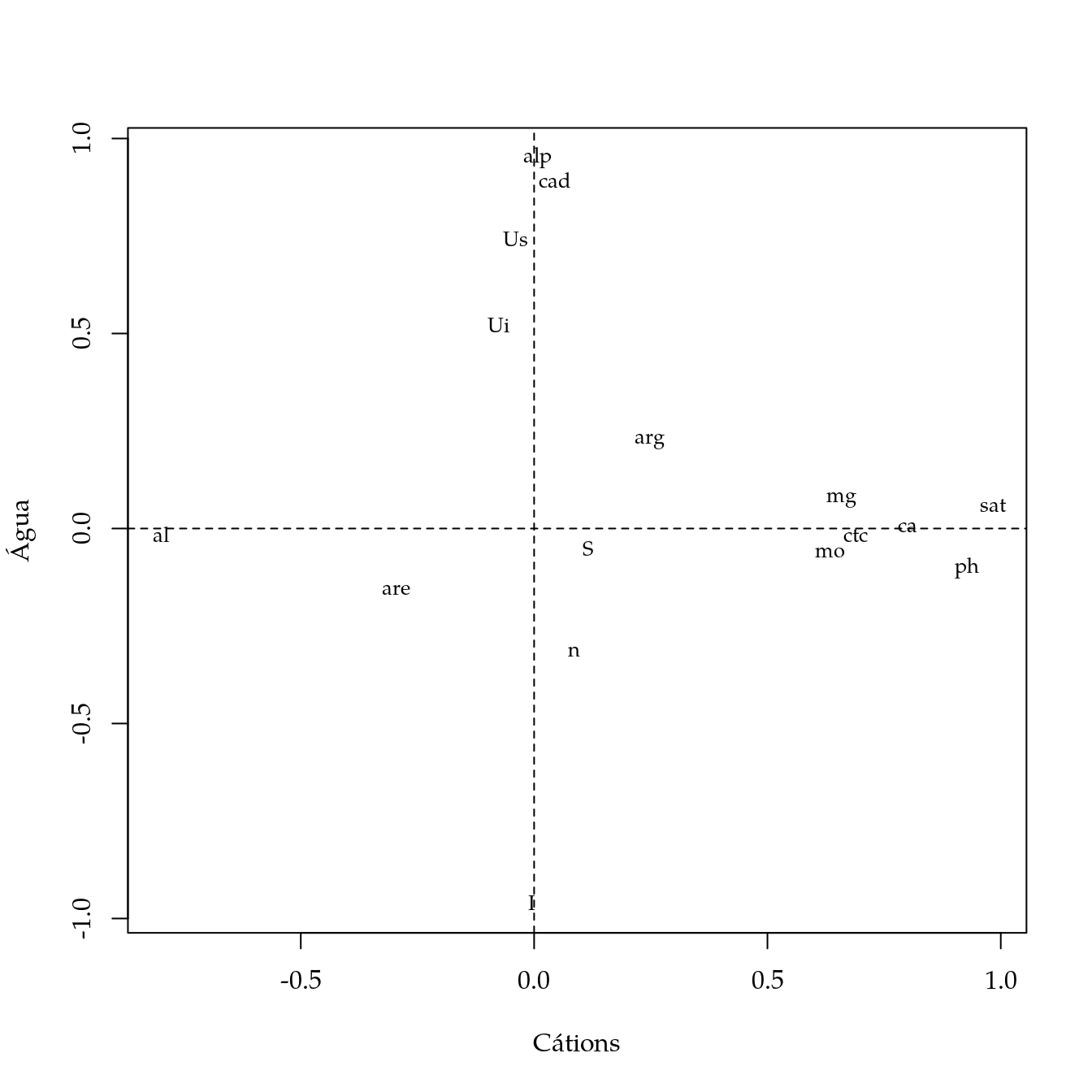
# Pares de gráficos dos escores.
sc <- fit1$scores
pairs(sc)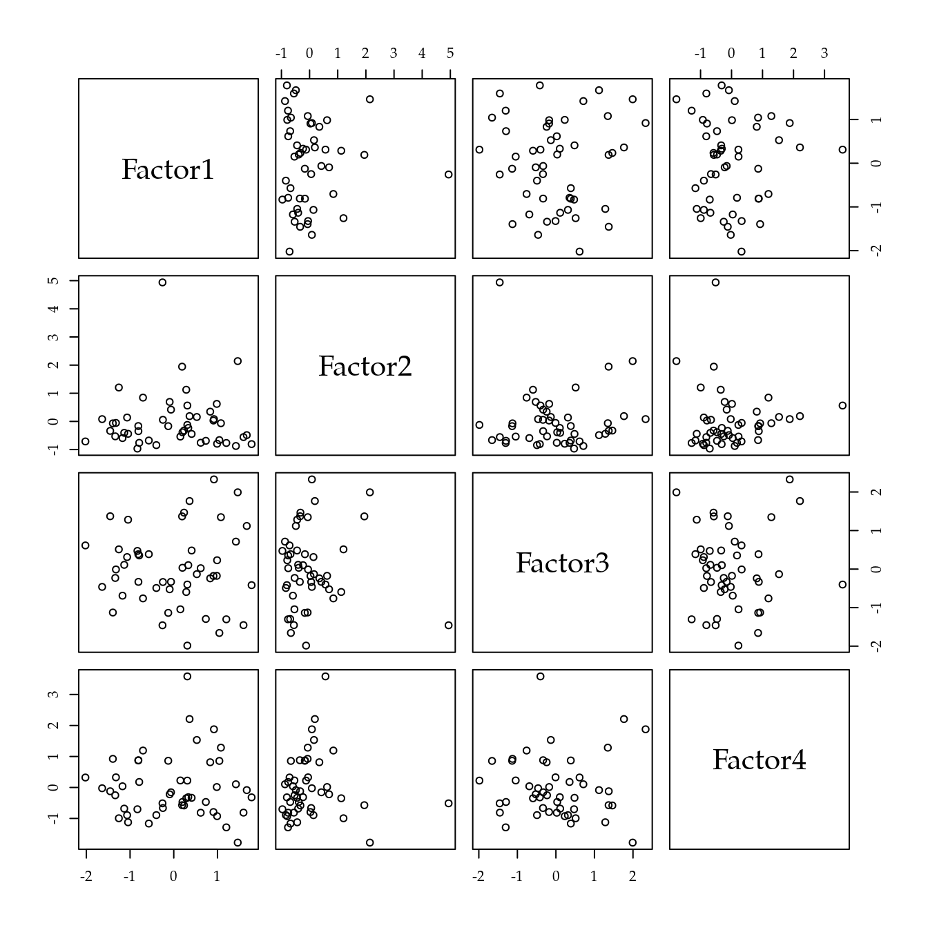
Os resultados com o abandono das variáveis de alta singularidade não sofreu modificações substanciais. A interpretação dos fatores foi mantida. Com estes 4 fatores foi obtido uma explicação de 80% da variância total.
Apenas por precaução, foi confirmado por simulação que o número de fatores é de fato 4.
#-----------------------------------------------------------------------
# Determinação por simulação do número de fatores.

ev <- eigen(cor(X))
ap <- parallel(subject = nrow(X),
               var = ncol(X),
               rep = 100,
               cent = 0.05)

nS <- nScree(x = ev$values, aparallel = ap$eigen$qevpea)
plotnScree(nS)
Ajuste de Modelo de Regressão com os Escores
Os escores ou índices definidos pela análise fatorial serão usados como variáveis explicativas da produção de madeira.
#-----------------------------------------------------------------------
# Justar os escores com a variável de produção de madeira.

de <- merge(cbind(loc = dd[, "loc"], as.data.frame(sc)),
            teca_arv[, c("loc", "prod")])
names(de)[2:5] <- colnames(fit1$loadings)
str(de)
## 'data.frame': 49 obs. of 6 variables:
## $ loc : int 1 2 3 4 5 6 7 8 9 10 ...
## $ cation: num 1.043 -1.393 1.202 0.31 -0.809 ...
## $ agua : num -0.6641 -0.0693 -0.7665 -0.1251 -0.3466 ...
## $ poros : num -1.657 -1.127 -1.303 -1.985 -0.332 ...
## $ inclin: num 0.856 0.923 -1.287 0.222 0.879 ...
## $ prod : num 68.2 24.3 125.3 102.7 54.6 ...xyplot(sqrt(prod) ~ cation + agua + poros + inclin,
data = de,
outer = TRUE,
type = c("p", "r"),
as.table = TRUE,
scales = list(x = list(relation = "free")),
xlab = "Escores da análise fatorial",
ylab = "Produção de madeira")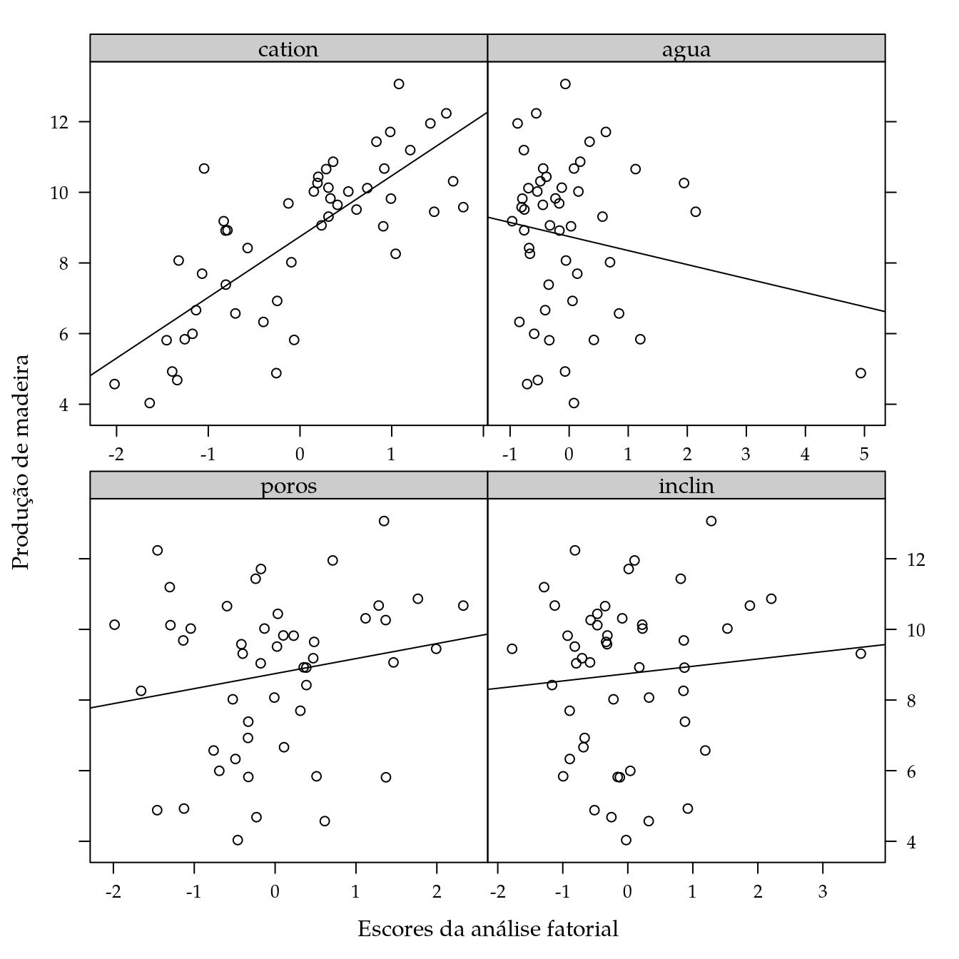
#-----------------------------------------------------------------------
# Ajuste do modelo de regressão.

# ATTENTION: Existe um maior atendimento dos pressupostos usando sqrt do
# que a variável original.

# m0 <- lm(prod ~ . - loc, data = de)
m0 <- lm(sqrt(prod) ~ . - loc, data = de)
summary(m0)
##
## Call:
## lm(formula = sqrt(prod) ~ . - loc, data = de)
##
## Residuals:
## Min 1Q Median 3Q Max
## -2.4828 -1.0219 -0.1136 1.1849 3.2479
##
## Coefficients:
## Estimate Std. Error t value Pr(>|t|)
## (Intercept) 8.7482 0.1970 44.397 < 2e-16 ***
## cation 1.7179 0.2005 8.567 6.28e-11 ***
## agua -0.3986 0.1997 -1.996 0.0521 .
## poros 0.4118 0.2028 2.030 0.0484 *
## inclin 0.2033 0.1996 1.019 0.3140
## ---
## Signif. codes: 0 '***' 0.001 '**' 0.01 '*' 0.05 '.' 0.1 ' ' 1
##
## Residual standard error: 1.379 on 44 degrees of freedom
## Multiple R-squared: 0.6531, Adjusted R-squared: 0.6216
## F-statistic: 20.71 on 4 and 44 DF, p-value: 1.178e-09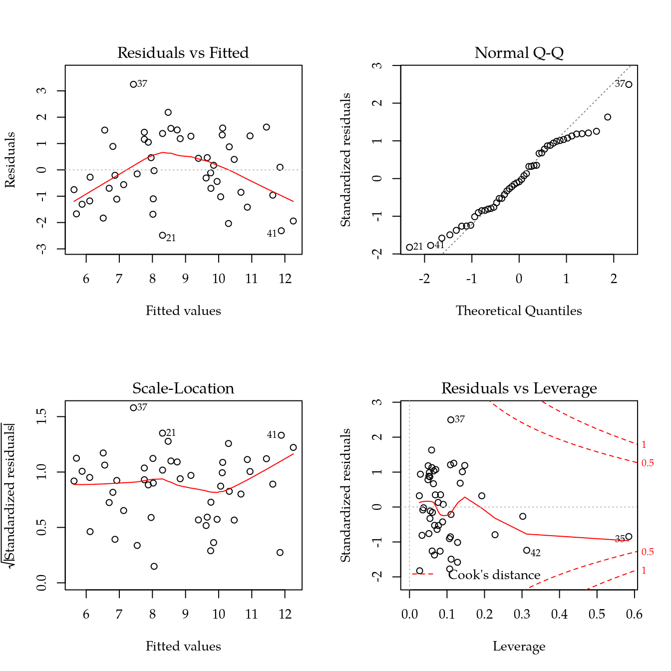
layout(1)

# MASS::boxcox(m0)
# abline(v = c(0.5, 1), col = 2)

residualPlots(m0)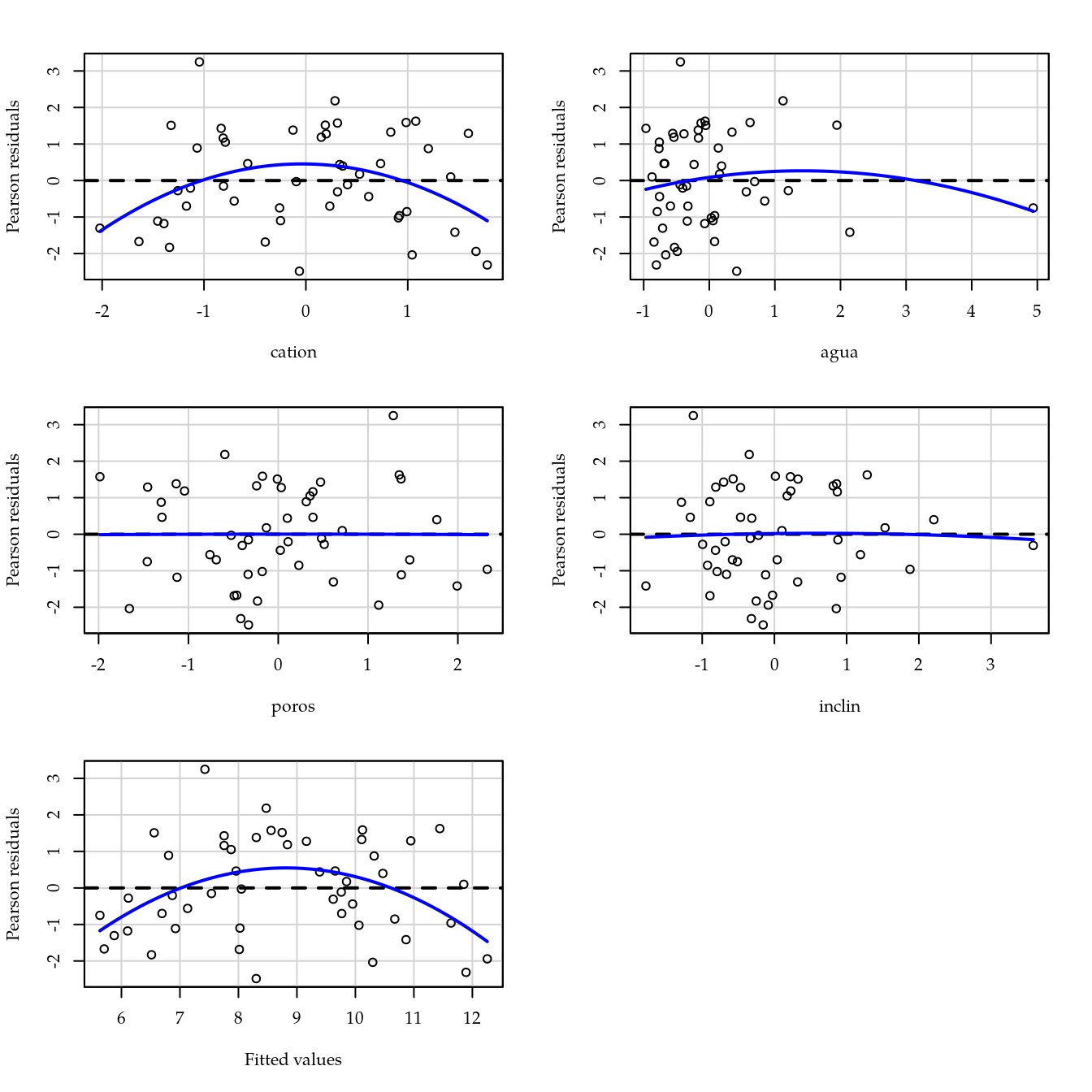
##            Test stat Pr(>|Test stat|)
## cation       -2.5355         0.014947 *
## agua         -1.0037         0.321149
## poros        -0.0227         0.982007
## inclin       -0.1624         0.871744
## Tukey test   -3.1528         0.001617 **
## ---
## Signif. codes:  0 '***' 0.001 '**' 0.01 '*' 0.05 '.' 0.1 ' ' 1
im <- influence.measures(m0)
summary(im)## Potentially influential observations of
## lm(formula = sqrt(prod) ~ . - loc, data = de) :
##
## dfb.1_ dfb.catn dfb.agua dfb.pors dfb.incl dffit cov.r cook.d
## 12 -0.05 -0.01 -0.03 0.02 -0.16 -0.17 1.59_* 0.01
## 35 -0.19 0.05 -0.93 0.28 0.09 -1.00 2.49_* 0.20
## 37 0.40 -0.43 -0.18 0.54 -0.46 0.94 0.59_* 0.15
## 42 -0.21 -0.32 -0.46 -0.44 0.39 -0.84 1.37_* 0.14
## 47 -0.13 -0.12 -0.01 -0.31 -0.24 -0.43 1.35_* 0.04
## 48 0.05 0.02 0.01 0.09 0.11 0.16 1.37_* 0.00
## hat
## 12 0.30
## 35 0.58_*
## 37 0.11
## 42 0.31_*
## 47 0.23
## 48 0.19# Remover observação com maior alavancagem.
which(im$is.inf[, "hat"])## 35 42
## 35 42r <- which.max(im$infmat[, "hat"])
m0 <- lm(prod ~ . - loc, data = de[-r, ])
# m0 <- lm(sqrt(prod) ~ . - loc, data = de[, 35])
summary(m0)##
## Call:
## lm(formula = prod ~ . - loc, data = de[-r, ])
##
## Residuals:
## Min 1Q Median 3Q Max
## -41.983 -14.926 -4.481 18.769 56.312
##
## Coefficients:
## Estimate Std. Error t value Pr(>|t|)
## (Intercept) 81.883 3.477 23.547 < 2e-16 ***
## cation 28.370 3.460 8.199 2.48e-10 ***
## agua -3.858 5.140 -0.750 0.457
## poros 6.110 3.686 1.658 0.105
## inclin 3.659 3.461 1.057 0.296
## ---
## Signif. codes: 0 '***' 0.001 '**' 0.01 '*' 0.05 '.' 0.1 ' ' 1
##
## Residual standard error: 23.76 on 43 degrees of freedom
## Multiple R-squared: 0.6216, Adjusted R-squared: 0.5864
## F-statistic: 17.66 on 4 and 43 DF, p-value: 1.21e-08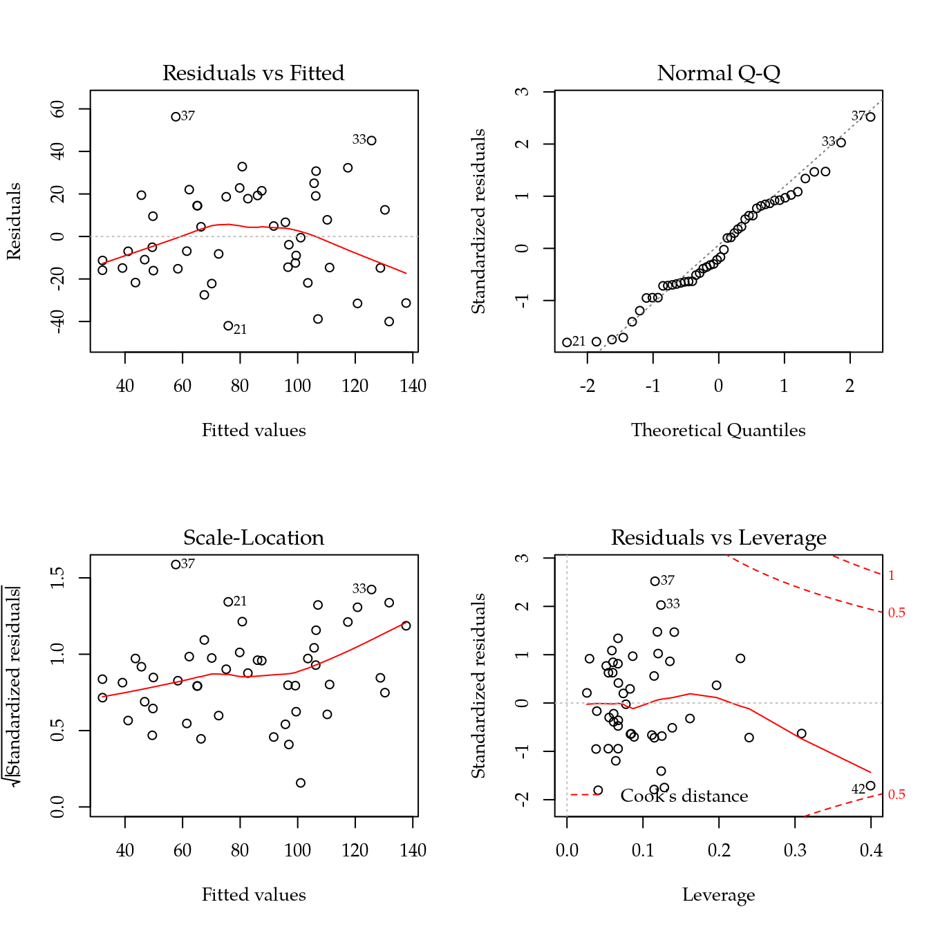
layout(1)

residualPlots(m0)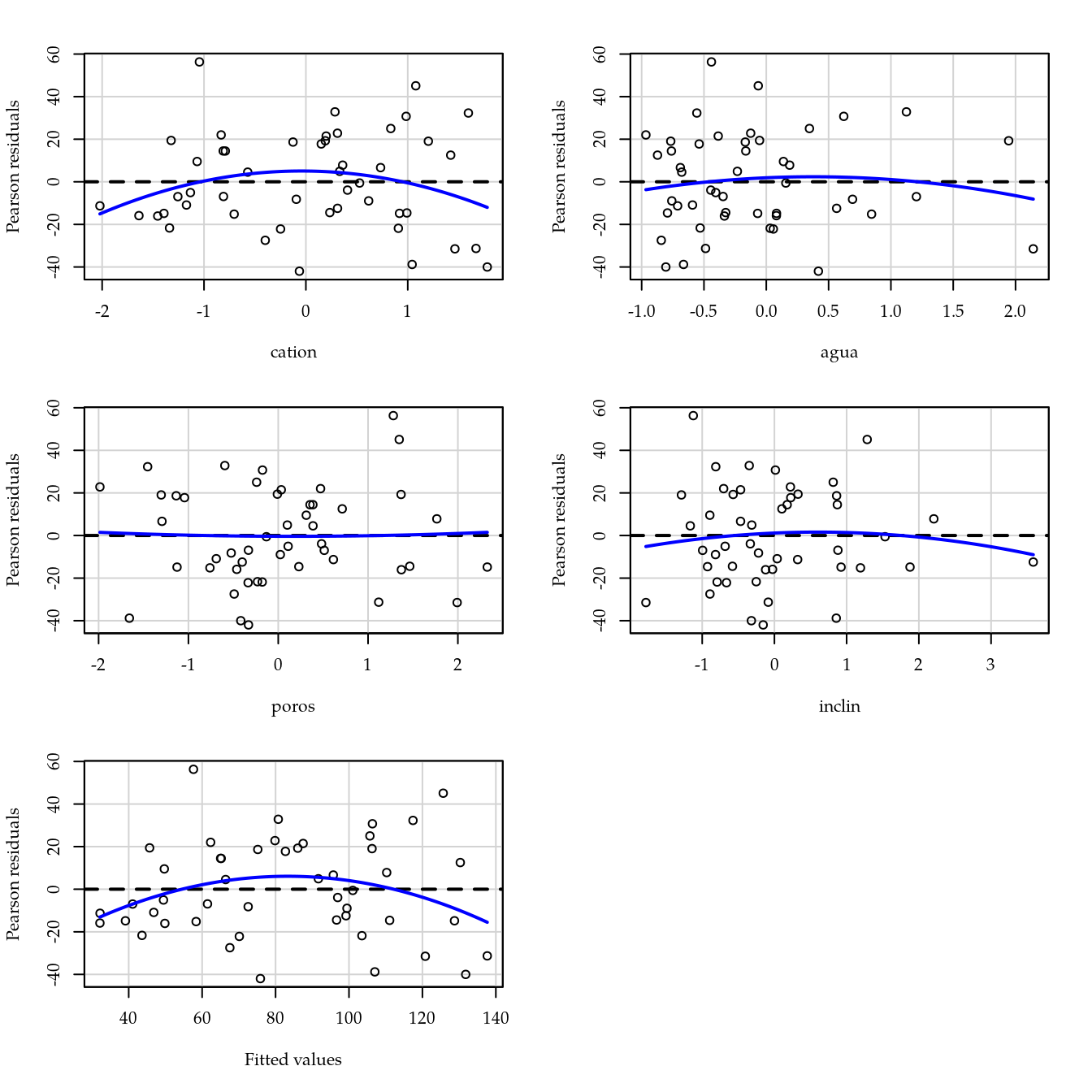
##            Test stat Pr(>|Test stat|)
## cation       -1.5154          0.13717
## agua         -0.7977          0.42953
## poros         0.1490          0.88229
## inclin       -0.5833          0.56278
## Tukey test   -1.9140          0.05562 .
## ---
## Signif. codes: 0 '***' 0.001 '**' 0.01 '*' 0.05 '.' 0.1 ' ' 1##
## Call:
## lm(formula = prod ~ cation, data = de[-r, ])
##
## Residuals:
## Min 1Q Median 3Q Max
## -46.818 -16.356 -0.935 19.611 60.985
##
## Coefficients:
## Estimate Std. Error t value Pr(>|t|)
## (Intercept) 82.505 3.461 23.84 < 2e-16 ***
## cation 28.256 3.489 8.10 2.11e-10 ***
## ---
## Signif. codes: 0 '***' 0.001 '**' 0.01 '*' 0.05 '.' 0.1 ' ' 1
##
## Residual standard error: 23.98 on 46 degrees of freedom
## Multiple R-squared: 0.5878, Adjusted R-squared: 0.5789
## F-statistic: 65.61 on 1 and 46 DF, p-value: 2.109e-10anova(m0, m1)## Analysis of Variance Table
##
## Model 1: prod ~ (loc + cation + agua + poros + inclin) - loc
## Model 2: prod ~ cation
## Res.Df RSS Df Sum of Sq F Pr(>F)
## 1 43 24285
## 2 46 26453 -3 -2168.3 1.2798 0.2934# Carregamento das variáveis no fator 1.
cbind(fit1$loadings[, "cation"])## [,1]
## ph 0.926568323
## ca 0.799790530
## mg 0.657556973
## al -0.799126322
## ctc 0.689678273
## sat 0.983762102
## mo 0.633119567
## arg 0.247663547
## are -0.295782957
## alp 0.007755497
## n 0.085257262
## I -0.005033060
## Us -0.040342066
## Ui -0.075900927
## S 0.115606042
## cad 0.044470468Ajuste de Modelo de Regressão Múltipla com a Variáveis de Solo
#-----------------------------------------------------------------------

de <- merge(subset(dd, select = -cam),
            teca_arv[, c("loc", "prod")])
de <- subset(de, select = -loc)
str(de)
## 'data.frame': 49 obs. of 22 variables:
## $ ph : num 6.7 4.7 6.8 6.2 5.1 5.2 5.1 6.4 4.9 5 ...
## $ p : num 0.83 0.69 1.66 1.17 0.49 0.69 0.21 1.14 1.36 1.04 ...
## $ k : num 13.4 12.3 25.8 11.1 22.2 ...
## $ ca : num 2.91 0.76 3.22 2.25 0.93 0.7 0.24 2.39 1.15 0.72 ...
## $ mg : num 1.77 0.14 1.31 0.21 0.52 0.36 0.14 0.99 0.05 0.37 ...
## $ al : num 0 0.6 0 0 0.2 0.5 0.6 0 0.3 0.6 ...
## $ ctc : num 6.57 4.17 6.26 4.56 4.1 5.16 5.02 5.28 4.86 3.86 ...
## $ sat : num 71.7 22.4 73.4 54.5 36.8 ...
## $ mo : num 25.6 8.7 15.6 10 11.2 5.8 8.5 11.8 6.3 6.9 ...
## $ arg : num 215 213 234 169 304 ...
## $ are : num 750 775 698 788 665 ...
## $ cas : num 2.2 1.1 19 3.1 7.2 23.4 2.9 2.1 2.5 1.6 ...
## $ acc : num 750 775 704 788 667 ...
## $ Ur : num 0.1785 0.1649 0.3699 0.0372 0.1902 ...
## $ Us : num 0.58 0.573 0.659 0.521 0.608 ...
## $ alp : num -0.833 -0.547 -0.552 -0.478 -0.671 ...
## $ n : num 3.11 2.92 1.96 2.21 2.93 ...
## $ I : num 0.957 0.691 0.918 0.751 0.813 ...
## $ Ui : num 0.396 0.387 0.538 0.311 0.418 ...
## $ S : num 0.273 0.257 0.108 0.214 0.265 ...
## $ cad : num 0.217 0.222 0.168 0.274 0.228 ...
## $ prod: num 68.2 24.3 125.3 102.7 54.6 ...# Número de observações.
nrow(de)## [1] 49## Analysis of Variance Table
##
## Response: sqrt(prod)
## Df Sum Sq Mean Sq F value Pr(>F)
## ph 1 121.034 121.034 64.7234 9.248e-09 ***
## p 1 0.001 0.001 0.0003 0.985446
## k 1 0.511 0.511 0.2734 0.605170
## ca 1 1.671 1.671 0.8937 0.352563
## mg 1 8.111 8.111 4.3376 0.046532 *
## al 1 17.593 17.593 9.4080 0.004753 **
## ctc 1 0.077 0.077 0.0414 0.840253
## sat 1 8.074 8.074 4.3179 0.046998 *
## mo 1 0.336 0.336 0.1799 0.674721
## arg 1 6.766 6.766 3.6184 0.067477 .
## are 1 0.617 0.617 0.3302 0.570150
## cas 1 6.252 6.252 3.3434 0.078148 .
## acc 1 6.342 6.342 3.3916 0.076146 .
## Ur 1 2.965 2.965 1.5858 0.218324
## Us 1 7.533 7.533 4.0284 0.054482 .
## alp 1 0.054 0.054 0.0291 0.865882
## n 1 0.066 0.066 0.0355 0.851830
## I 1 0.064 0.064 0.0341 0.854905
## Ui 1 0.335 0.335 0.1790 0.675461
## S 1 0.541 0.541 0.2891 0.595043
## Residuals 28 52.360 1.870
## ---
## Signif. codes: 0 '***' 0.001 '**' 0.01 '*' 0.05 '.' 0.1 ' ' 1# im <- influence.measures(m0)
# summary(im)
# residualPlots(m0)
# AIC.
m1 <- step(m0)## Start: AIC=45.25
## sqrt(prod) ~ ph + p + k + ca + mg + al + ctc + sat + mo + arg +
## are + cas + acc + Ur + Us + alp + n + I + Ui + S + cad
##
##
## Step: AIC=45.25
## sqrt(prod) ~ ph + p + k + ca + mg + al + ctc + sat + mo + arg +
## are + cas + acc + Ur + Us + alp + n + I + Ui + S
##
## Df Sum of Sq RSS AIC
## - al 1 0.1091 52.469 43.352
## - ph 1 0.1360 52.496 43.377
## - p 1 0.1583 52.519 43.398
## - mo 1 0.1864 52.547 43.424
## - are 1 0.2754 52.636 43.507
## - acc 1 0.4390 52.799 43.659
## - mg 1 0.5026 52.863 43.718
## - S 1 0.5406 52.901 43.753
## - n 1 0.5551 52.915 43.767
## - k 1 0.5907 52.951 43.800
## - Us 1 0.6722 53.032 43.875
## - ctc 1 0.7027 53.063 43.903
## - I 1 0.7352 53.096 43.933
## - alp 1 0.7678 53.128 43.963
## - cas 1 0.7871 53.147 43.981
## - Ui 1 0.8273 53.188 44.018
## - Ur 1 1.1022 53.463 44.271
## - arg 1 1.4390 53.799 44.579
## <none> 52.360 45.250
## - ca 1 2.5508 54.911 45.581
## - sat 1 8.6951 61.055 50.778
##
## Step: AIC=43.35
## sqrt(prod) ~ ph + p + k + ca + mg + ctc + sat + mo + arg + are +
## cas + acc + Ur + Us + alp + n + I + Ui + S
##
## Df Sum of Sq RSS AIC
## - p 1 0.1535 52.623 41.495
## - mo 1 0.1872 52.657 41.527
## - ph 1 0.1899 52.659 41.529
## - are 1 0.3594 52.829 41.687
## - acc 1 0.4626 52.932 41.782
## - k 1 0.7087 53.178 42.010
## - cas 1 0.8075 53.277 42.100
## - mg 1 0.9644 53.434 42.245
## - S 1 1.0394 53.509 42.313
## - n 1 1.1012 53.571 42.370
## - Us 1 1.1784 53.648 42.440
## - ctc 1 1.2259 53.695 42.484
## - I 1 1.2473 53.717 42.503
## - alp 1 1.2807 53.750 42.534
## - arg 1 1.3416 53.811 42.589
## - Ui 1 1.3832 53.853 42.627
## - Ur 1 1.7026 54.172 42.917
## <none> 52.469 43.352
## - ca 1 4.3899 56.859 45.289
## - sat 1 26.3415 78.811 61.286
##
## Step: AIC=41.5
## sqrt(prod) ~ ph + k + ca + mg + ctc + sat + mo + arg + are +
## cas + acc + Ur + Us + alp + n + I + Ui + S
##
## Df Sum of Sq RSS AIC
## - mo 1 0.2383 52.861 39.717
## - are 1 0.2393 52.862 39.718
## - ph 1 0.2486 52.872 39.726
## - acc 1 0.3266 52.950 39.798
## - k 1 0.5601 53.183 40.014
## - cas 1 0.6551 53.278 40.101
## - mg 1 0.9994 53.622 40.417
## - S 1 1.0411 53.664 40.455
## - n 1 1.1224 53.745 40.529
## - Us 1 1.2403 53.863 40.637
## - arg 1 1.2586 53.881 40.653
## - ctc 1 1.2874 53.910 40.680
## - I 1 1.3524 53.975 40.739
## - alp 1 1.3817 54.005 40.765
## - Ui 1 1.4679 54.091 40.843
## - Ur 1 1.8284 54.451 41.169
## <none> 52.623 41.495
## - ca 1 4.3406 56.964 43.379
## - sat 1 26.8594 79.482 59.702
##
## Step: AIC=39.72
## sqrt(prod) ~ ph + k + ca + mg + ctc + sat + arg + are + cas +
## acc + Ur + Us + alp + n + I + Ui + S
##
## Df Sum of Sq RSS AIC
## - are 1 0.1667 53.028 37.871
## - acc 1 0.2154 53.077 37.916
## - ph 1 0.3069 53.168 38.000
## - k 1 0.3825 53.244 38.070
## - cas 1 0.5328 53.394 38.208
## - mg 1 0.8962 53.757 38.540
## - S 1 1.1422 54.003 38.764
## - ctc 1 1.1804 54.042 38.799
## - arg 1 1.1847 54.046 38.803
## - n 1 1.2248 54.086 38.839
## - Us 1 1.3415 54.203 38.945
## - I 1 1.4405 54.302 39.034
## - alp 1 1.4420 54.303 39.035
## - Ui 1 1.5623 54.423 39.144
## - Ur 1 1.8994 54.761 39.446
## <none> 52.861 39.717
## - ca 1 4.1151 56.976 41.390
## - sat 1 26.6450 79.506 57.717
##
## Step: AIC=37.87
## sqrt(prod) ~ ph + k + ca + mg + ctc + sat + arg + cas + acc +
## Ur + Us + alp + n + I + Ui + S
##
## Df Sum of Sq RSS AIC
## - acc 1 0.0488 53.077 35.916
## - ph 1 0.2359 53.264 36.088
## - k 1 0.3874 53.415 36.228
## - cas 1 0.5930 53.621 36.416
## - mg 1 0.9841 54.012 36.772
## - S 1 0.9917 54.020 36.779
## - n 1 1.0683 54.096 36.848
## - Us 1 1.1997 54.228 36.967
## - ctc 1 1.2445 54.272 37.007
## - I 1 1.2845 54.312 37.044
## - alp 1 1.2888 54.317 37.048
## - Ui 1 1.4179 54.446 37.164
## - Ur 1 1.7630 54.791 37.473
## <none> 53.028 37.871
## - arg 1 2.8066 55.834 38.398
## - ca 1 3.9563 56.984 39.397
## - sat 1 28.2845 81.312 56.817
##
## Step: AIC=35.92
## sqrt(prod) ~ ph + k + ca + mg + ctc + sat + arg + cas + Ur +
## Us + alp + n + I + Ui + S
##
## Df Sum of Sq RSS AIC
## - ph 1 0.2831 53.360 34.177
## - k 1 0.4963 53.573 34.372
## - mg 1 0.9388 54.015 34.775
## - ctc 1 1.2203 54.297 35.030
## - S 1 1.3278 54.404 35.127
## - cas 1 1.3634 54.440 35.159
## - n 1 1.4218 54.498 35.211
## - Us 1 1.4591 54.536 35.245
## - alp 1 1.4782 54.555 35.262
## - I 1 1.5151 54.592 35.295
## - Ui 1 1.6751 54.752 35.438
## - Ur 1 1.9689 55.045 35.701
## <none> 53.077 35.916
## - ca 1 3.9535 57.030 37.436
## - arg 1 7.1858 60.262 40.138
## - sat 1 28.4168 81.493 54.926
##
## Step: AIC=34.18
## sqrt(prod) ~ k + ca + mg + ctc + sat + arg + cas + Ur + Us +
## alp + n + I + Ui + S
##
## Df Sum of Sq RSS AIC
## - k 1 0.640 53.999 32.760
## - mg 1 1.176 54.536 33.245
## - S 1 1.259 54.618 33.319
## - n 1 1.377 54.737 33.425
## - Us 1 1.426 54.786 33.469
## - alp 1 1.439 54.799 33.481
## - I 1 1.474 54.834 33.512
## - ctc 1 1.527 54.887 33.559
## - cas 1 1.560 54.919 33.588
## - Ui 1 1.626 54.985 33.647
## - Ur 1 1.902 55.262 33.893
## <none> 53.360 34.177
## - ca 1 4.656 58.016 36.276
## - arg 1 7.357 60.717 38.506
## - sat 1 34.002 87.362 56.334
##
## Step: AIC=32.76
## sqrt(prod) ~ ca + mg + ctc + sat + arg + cas + Ur + Us + alp +
## n + I + Ui + S
##
## Df Sum of Sq RSS AIC
## - S 1 1.049 55.048 31.703
## - Us 1 1.190 55.189 31.829
## - n 1 1.219 55.219 31.855
## - alp 1 1.261 55.260 31.892
## - I 1 1.303 55.303 31.929
## - Ui 1 1.381 55.380 31.998
## - mg 1 1.391 55.391 32.007
## - ctc 1 1.450 55.449 32.059
## - Ur 1 1.636 55.636 32.223
## - cas 1 1.897 55.897 32.453
## <none> 53.999 32.760
## - ca 1 4.603 58.602 34.768
## - arg 1 8.631 62.630 38.026
## - sat 1 33.364 87.363 54.334
##
## Step: AIC=31.7
## sqrt(prod) ~ ca + mg + ctc + sat + arg + cas + Ur + Us + alp +
## n + I + Ui
##
## Df Sum of Sq RSS AIC
## - Us 1 0.148 55.197 29.835
## - alp 1 0.252 55.300 29.927
## - I 1 0.273 55.321 29.945
## - Ui 1 0.332 55.381 29.998
## - n 1 0.380 55.428 30.040
## - Ur 1 0.589 55.637 30.224
## - ctc 1 1.036 56.084 30.617
## - mg 1 1.339 56.387 30.881
## - cas 1 2.011 57.059 31.461
## <none> 55.048 31.703
## - ca 1 3.840 58.888 33.007
## - arg 1 10.476 65.525 38.240
## - sat 1 32.436 87.484 52.402
##
## Step: AIC=29.84
## sqrt(prod) ~ ca + mg + ctc + sat + arg + cas + Ur + alp + n +
## I + Ui
##
## Df Sum of Sq RSS AIC
## - alp 1 0.173 55.370 27.988
## - I 1 0.190 55.387 28.003
## - n 1 0.317 55.514 28.116
## - ctc 1 1.062 56.259 28.769
## - mg 1 1.341 56.538 29.012
## - cas 1 1.991 57.188 29.571
## <none> 55.197 29.835
## - Ui 1 3.078 58.275 30.494
## - ca 1 4.269 59.466 31.485
## - Ur 1 4.544 59.740 31.711
## - arg 1 15.139 70.335 39.711
## - sat 1 34.637 89.834 51.701
##
## Step: AIC=27.99
## sqrt(prod) ~ ca + mg + ctc + sat + arg + cas + Ur + n + I + Ui
##
## Df Sum of Sq RSS AIC
## - I 1 0.019 55.389 26.005
## - n 1 0.145 55.515 26.117
## - ctc 1 0.974 56.344 26.843
## - mg 1 1.277 56.647 27.106
## <none> 55.370 27.988
## - cas 1 2.355 57.725 28.029
## - Ui 1 3.974 59.344 29.385
## - ca 1 4.106 59.476 29.494
## - Ur 1 5.475 60.844 30.608
## - arg 1 15.122 70.492 37.820
## - sat 1 35.426 90.795 50.222
##
## Step: AIC=26.01
## sqrt(prod) ~ ca + mg + ctc + sat + arg + cas + Ur + n + Ui
##
## Df Sum of Sq RSS AIC
## - n 1 0.143 55.532 24.132
## - ctc 1 1.040 56.429 24.917
## - mg 1 1.353 56.742 25.188
## <none> 55.389 26.005
## - cas 1 2.336 57.725 26.030
## - ca 1 4.090 59.479 27.496
## - Ui 1 9.757 65.146 31.956
## - Ur 1 13.046 68.435 34.369
## - arg 1 15.539 70.928 36.122
## - sat 1 35.929 91.318 48.504
##
## Step: AIC=24.13
## sqrt(prod) ~ ca + mg + ctc + sat + arg + cas + Ur + Ui
##
## Df Sum of Sq RSS AIC
## - ctc 1 0.957 56.489 22.969
## - mg 1 1.214 56.746 23.192
## - cas 1 2.297 57.828 24.117
## <none> 55.532 24.132
## - ca 1 3.964 59.496 25.510
## - Ur 1 14.922 70.454 33.794
## - Ui 1 14.940 70.472 33.807
## - arg 1 15.701 71.233 34.332
## - sat 1 36.137 91.669 46.692
##
## Step: AIC=22.97
## sqrt(prod) ~ ca + mg + sat + arg + cas + Ur + Ui
##
## Df Sum of Sq RSS AIC
## - mg 1 0.258 56.746 21.192
## - cas 1 1.850 58.338 22.548
## <none> 56.489 22.969
## - ca 1 9.953 66.442 28.921
## - Ui 1 16.720 73.208 33.673
## - Ur 1 17.982 74.471 34.511
## - arg 1 18.394 74.882 34.781
## - sat 1 61.160 117.649 56.918
##
## Step: AIC=21.19
## sqrt(prod) ~ ca + sat + arg + cas + Ur + Ui
##
## Df Sum of Sq RSS AIC
## - cas 1 1.997 58.743 20.887
## <none> 56.746 21.192
## - ca 1 9.731 66.477 26.947
## - Ui 1 16.470 73.216 31.678
## - Ur 1 17.751 74.497 32.528
## - arg 1 18.847 75.594 33.244
## - sat 1 77.056 133.802 61.223
##
## Step: AIC=20.89
## sqrt(prod) ~ ca + sat + arg + Ur + Ui
##
## Df Sum of Sq RSS AIC
## <none> 58.743 20.887
## - ca 1 8.928 67.671 25.819
## - arg 1 17.223 75.966 31.485
## - Ui 1 20.059 78.802 33.281
## - Ur 1 21.014 79.758 33.871
## - sat 1 75.715 134.458 59.462# Resumo do modelo selecionado.
summary(m1)##
## Call:
## lm(formula = sqrt(prod) ~ ca + sat + arg + Ur + Ui, data = de)
##
## Residuals:
## Min 1Q Median 3Q Max
## -2.74099 -0.70075 -0.07258 0.74942 2.61550
##
## Coefficients:
## Estimate Std. Error t value Pr(>|t|)
## (Intercept) 4.758265 1.553767 3.062 0.003779 **
## ca -0.373064 0.145932 -2.556 0.014190 *
## sat 0.108190 0.014533 7.445 2.94e-09 ***
## arg 0.009024 0.002542 3.551 0.000946 ***
## Ur 12.619160 3.217513 3.922 0.000311 ***
## Ui -13.805028 3.602733 -3.832 0.000409 ***
## ---
## Signif. codes: 0 '***' 0.001 '**' 0.01 '*' 0.05 '.' 0.1 ' ' 1
##
## Residual standard error: 1.169 on 43 degrees of freedom
## Multiple R-squared: 0.7566, Adjusted R-squared: 0.7283
## F-statistic: 26.73 on 5 and 43 DF, p-value: 3.521e-12# residualPlots(m1)
anova(m1, m0)## Analysis of Variance Table
##
## Model 1: sqrt(prod) ~ ca + sat + arg + Ur + Ui
## Model 2: sqrt(prod) ~ ph + p + k + ca + mg + al + ctc + sat + mo + arg +
## are + cas + acc + Ur + Us + alp + n + I + Ui + S + cad
## Res.Df RSS Df Sum of Sq F Pr(>F)
## 1 43 58.743
## 2 28 52.360 15 6.3831 0.2276 0.998im <- influence.measures(m1)
summary(im)## Potentially influential observations of
## lm(formula = sqrt(prod) ~ ca + sat + arg + Ur + Ui, data = de) :
##
## dfb.1_ dfb.ca dfb.sat dfb.arg dfb.Ur dfb.Ui dffit cov.r
## 3 -0.07 -0.02 0.07 -0.06 0.10 0.03 0.18 1.47_*
## 4 1.40_* 0.15 -0.04 -0.83 -1.17_* -0.36 1.98_* 0.55_*
## 19 0.48 0.91 -0.98 -0.55 -0.42 0.18 -1.16_* 0.51_*
## 21 -0.34 0.21 -0.12 -0.10 0.38 0.17 -0.71 0.51_*
## 30 0.07 0.10 -0.07 -0.11 0.01 -0.01 -0.13 1.45_*
## 35 0.14 0.02 -0.03 0.09 0.17 -0.25 -0.26 2.78_*
## 42 -0.19 0.36 -0.24 -0.04 -0.22 0.32 0.60 2.24_*
## cook.d hat
## 3 0.01 0.23
## 4 0.55 0.31
## 19 0.20 0.15
## 21 0.07 0.07
## 30 0.00 0.22
## 35 0.01 0.59_*
## 42 0.06 0.51_*
layout(1)Árvore de Regressão
#-----------------------------------------------------------------------
# Árvore de regressão.

layout(1)

ar <- rpart(prod ~ ., data = de, method = "anova")

summary(ar)
## Call:
## rpart(formula = prod ~ ., data = de, method = "anova")
## n= 49
##
## CP nsplit rel error xerror xstd
## 1 0.57305253 0 1.0000000 1.0341216 0.1752373
## 2 0.10577603 1 0.4269475 0.5994510 0.1334305
## 3 0.07699958 2 0.3211714 0.5775419 0.1155758
## 4 0.01000000 3 0.2441719 0.4446810 0.1040718
##
## Variable importance
## sat ph ca al ctc mg mo Ui
## 20 17 17 16 13 13 3 1
##
## Node number 1: 49 observations, complexity param=0.5730525
## mean=81.45595, MSE=1379.012
## left son=2 (23 obs) right son=3 (26 obs)
## Primary splits:
## sat < 53.17 to the left, improve=0.5730525, (0 missing)
## ph < 5.65 to the left, improve=0.5178576, (0 missing)
## mg < 0.635 to the left, improve=0.5153786, (0 missing)
## al < 0.05 to the right, improve=0.5021701, (0 missing)
## ca < 2.12 to the left, improve=0.4585303, (0 missing)
## Surrogate splits:
## ph < 5.65 to the left, agree=0.959, adj=0.913, (0 split)
## al < 0.05 to the right, agree=0.939, adj=0.870, (0 split)
## ca < 2.245 to the left, agree=0.918, adj=0.826, (0 split)
## mg < 0.635 to the left, agree=0.898, adj=0.783, (0 split)
## ctc < 5.61 to the left, agree=0.857, adj=0.696, (0 split)
##
## Node number 2: 23 observations, complexity param=0.105776
## mean=51.56746, MSE=658.0742
## left son=4 (10 obs) right son=5 (13 obs)
## Primary splits:
## mo < 9.15 to the left, improve=0.4722245, (0 missing)
## ca < 0.84 to the left, improve=0.3706763, (0 missing)
## sat < 29.435 to the left, improve=0.3378541, (0 missing)
## acc < 641.93 to the right, improve=0.2859104, (0 missing)
## cad < 0.2013866 to the right, improve=0.2581536, (0 missing)
## Surrogate splits:
## sat < 30.435 to the left, agree=0.913, adj=0.8, (0 split)
## ca < 0.84 to the left, agree=0.870, adj=0.7, (0 split)
## al < 0.25 to the right, agree=0.826, adj=0.6, (0 split)
## ph < 5.25 to the left, agree=0.739, adj=0.4, (0 split)
## ctc < 5.2 to the left, agree=0.739, adj=0.4, (0 split)
##
## Node number 3: 26 observations, complexity param=0.07699958
## mean=107.8958, MSE=527.4539
## left son=6 (16 obs) right son=7 (10 obs)
## Primary splits:
## sat < 72.085 to the left, improve=0.3793975, (0 missing)
## cas < 39.85 to the left, improve=0.2627179, (0 missing)
## ca < 3.135 to the left, improve=0.1745765, (0 missing)
## mg < 1.94 to the left, improve=0.1397742, (0 missing)
## k < 33.61 to the left, improve=0.1044545, (0 missing)
## Surrogate splits:
## ph < 6.75 to the left, agree=0.846, adj=0.6, (0 split)
## ca < 6.055 to the left, agree=0.846, adj=0.6, (0 split)
## ctc < 11.025 to the left, agree=0.808, adj=0.5, (0 split)
## mg < 2.66 to the left, agree=0.769, adj=0.4, (0 split)
## Ui < 0.5205158 to the left, agree=0.731, adj=0.3, (0 split)
##
## Node number 4: 10 observations
## mean=31.46805, MSE=151.4165
##
## Node number 5: 13 observations
## mean=67.02855, MSE=498.0069
##
## Node number 6: 16 observations
## mean=96.71222, MSE=153.9737
##
## Node number 7: 10 observations
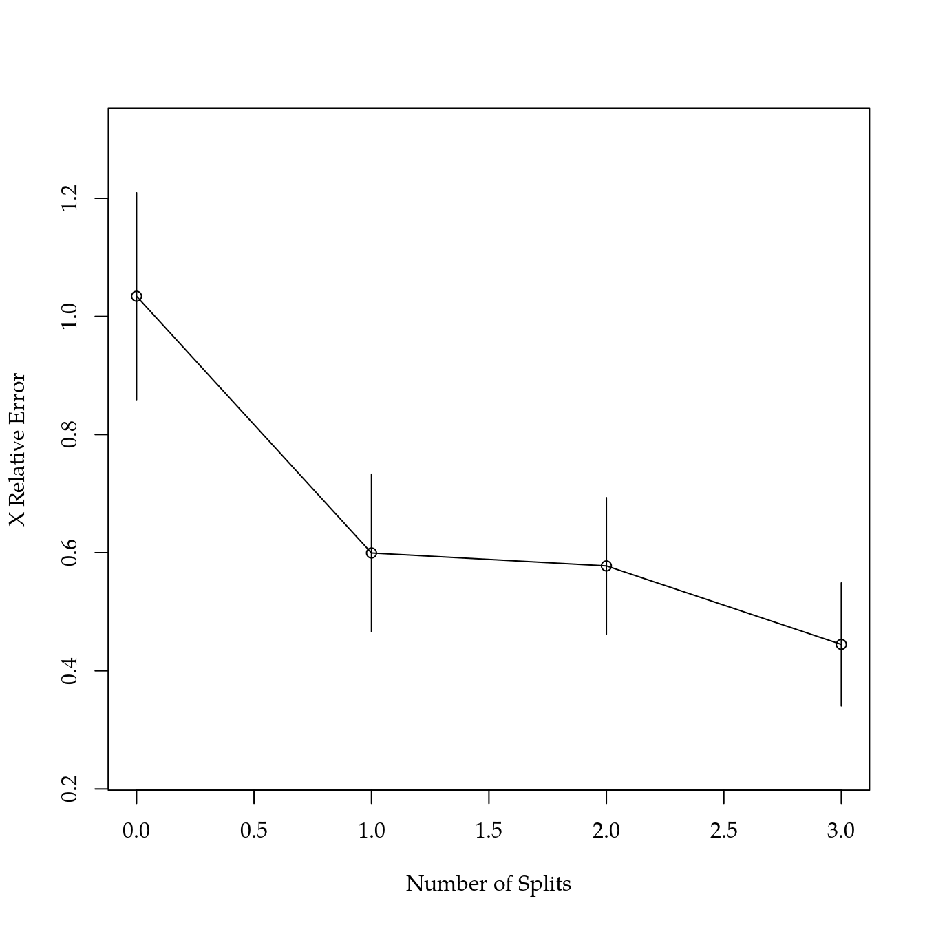
## mean=125.7894, MSE=604.7241rsq.rpart(ar)##
## Regression tree:
## rpart(formula = prod ~ ., data = de, method = "anova")
##
## Variables actually used in tree construction:
## [1] mo sat
##
## Root node error: 67572/49 = 1379
##
## n= 49
##
## CP nsplit rel error xerror xstd
## 1 0.57305 0 1.00000 1.03412 0.17524
## 2 0.10578 1 0.42695 0.59945 0.13343
## 3 0.07700 2 0.32117 0.57754 0.11558
## 4 0.01000 3 0.24417 0.44468 0.10407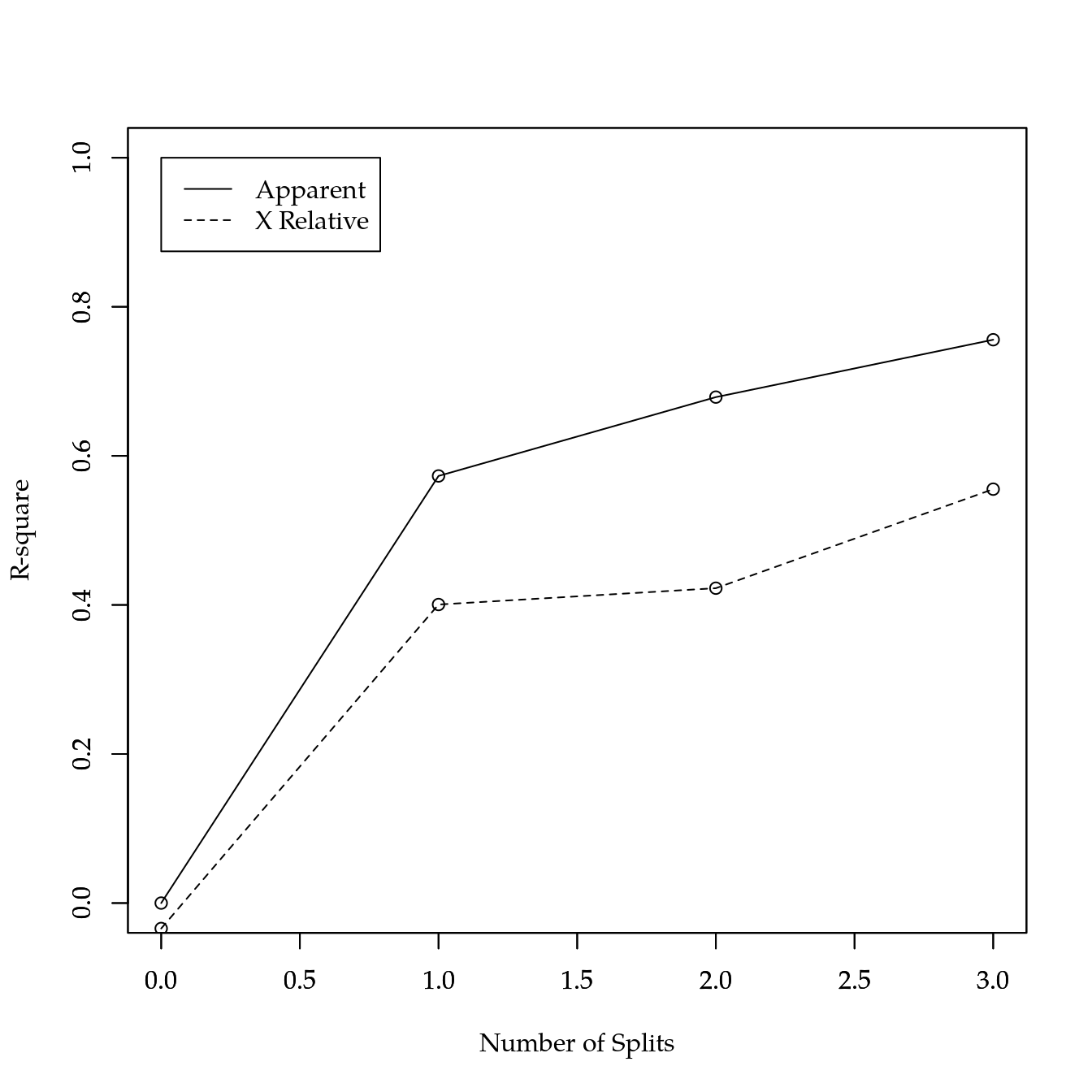
plot(ar, uniform = TRUE, main = "Árvore de regressão para produção")
text(ar, use.n = TRUE, all = TRUE, cex = 0.8)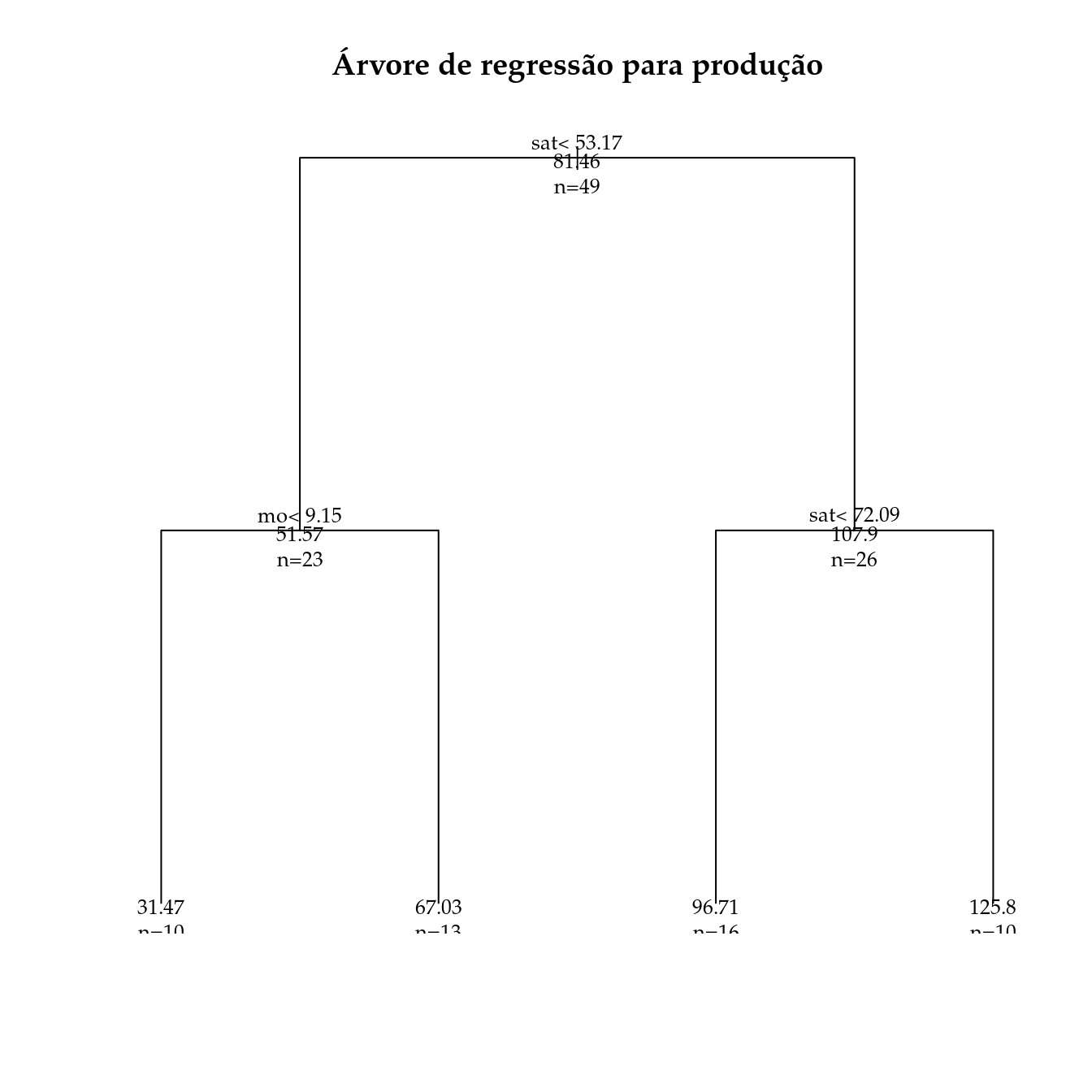
pred <- factor(predict(ar))
plot(sat ~ mo,
     data = de,
     col = as.integer(pred),
     pch = NA)
with(de, text(y = sat,
              x = mo,
              labels = rownames(de),
              col = as.integer(pred)))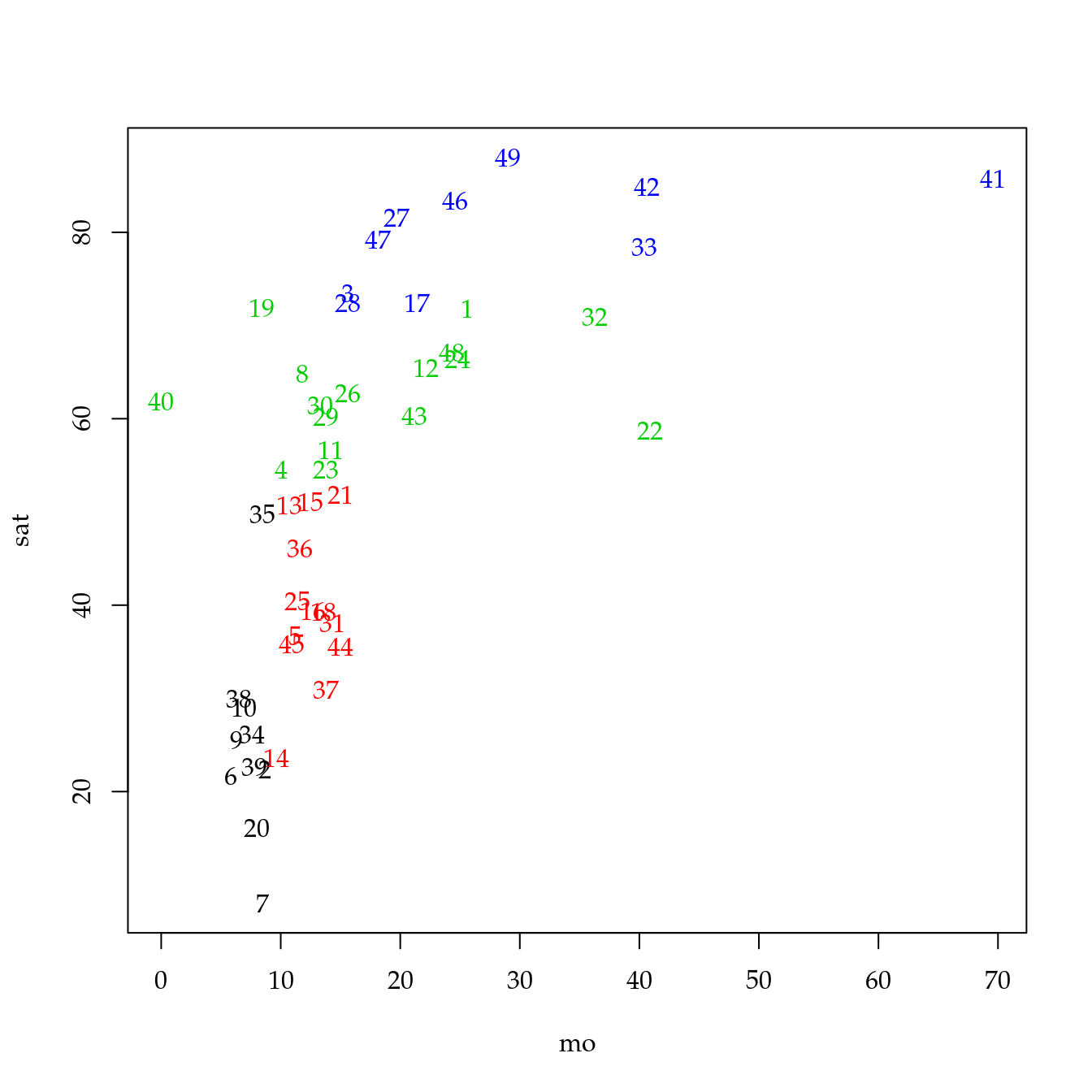
Informações da Sessão
## Atualizado em 11 de julho de 2019.
##
## R version 3.6.1 (2019-07-05)
## Platform: x86_64-pc-linux-gnu (64-bit)
## Running under: Ubuntu 18.04.2 LTS
##
## Matrix products: default
## BLAS:   /usr/lib/x86_64-linux-gnu/blas/libblas.so.3.7.1
## LAPACK: /usr/lib/x86_64-linux-gnu/lapack/liblapack.so.3.7.1
##
## locale:
##  [1] LC_CTYPE=pt_BR.UTF-8       LC_NUMERIC=C
##  [3] LC_TIME=pt_BR.UTF-8        LC_COLLATE=en_US.UTF-8
##  [5] LC_MONETARY=pt_BR.UTF-8    LC_MESSAGES=en_US.UTF-8
##  [7] LC_PAPER=pt_BR.UTF-8       LC_NAME=C
##  [9] LC_ADDRESS=C               LC_TELEPHONE=C
## [11] LC_MEASUREMENT=pt_BR.UTF-8 LC_IDENTIFICATION=C
##
## attached base packages:
## [1] stats     graphics  grDevices utils     datasets  methods
## [7] base
##
## other attached packages:
##  [1] rpart_4.1-15        nFactors_2.3.3      boot_1.3-23
##  [4] psych_1.8.12        MASS_7.3-51.4       car_3.0-3
##  [7] carData_3.0-2       reshape2_1.4.3      plyr_1.8.4
## [10] EACS_0.0-7          wzRfun_0.91         captioner_2.2.3
## [13] latticeExtra_0.6-28 RColorBrewer_1.1-2  lattice_0.20-38
## [16] knitr_1.23
##
## loaded via a namespace (and not attached):
##  [1] Rcpp_1.0.1        prettyunits_1.0.2 ps_1.3.0
##  [4] assertthat_0.2.1  zeallot_0.1.0     rprojroot_1.3-2
##  [7] digest_0.6.20     R6_2.4.0          cellranger_1.1.0
## [10] backports_1.1.4   evaluate_0.14     pillar_1.4.2
## [13] rlang_0.4.0       curl_3.3          readxl_1.3.1
## [16] rstudioapi_0.10   data.table_1.12.2 callr_3.3.0
## [19] rmarkdown_1.13    pkgdown_1.3.0     desc_1.2.0
## [22] devtools_2.1.0    stringr_1.4.0     foreign_0.8-71
## [25] compiler_3.6.1    xfun_0.8          pkgconfig_2.0.2
## [28] mnormt_1.5-5      pkgbuild_1.0.3    htmltools_0.3.6
## [31] tibble_2.1.3      roxygen2_6.1.1    rio_0.5.16
## [34] crayon_1.3.4      withr_2.1.2       commonmark_1.7
## [37] grid_3.6.1        nlme_3.1-140      magrittr_1.5
## [40] zip_2.0.3         cli_1.1.0         stringi_1.4.3
## [43] fs_1.3.1          remotes_2.1.0     testthat_2.1.1
## [46] xml2_1.2.0        vctrs_0.2.0       openxlsx_4.1.0.1
## [49] tools_3.6.1       forcats_0.4.0     glue_1.3.1
## [52] hms_0.5.0         parallel_3.6.1    abind_1.4-5
## [55] processx_3.4.0    pkgload_1.0.2     yaml_2.2.0
## [58] sessioninfo_1.1.1 memoise_1.1.0     haven_2.1.1
## [61] usethis_1.5.1