Análise do NDVI e a relação com a produtividade de Teca
Walmes M. Zeviani & Milson E. Serafim
Source:vignettes/teca_ndvi.Rmd
teca_ndvi.RmdAnálise Exploratória
#-----------------------------------------------------------------------
# Carrega os pacotes necessários.

library(EACS)
library(tidyverse)
# Conversão para `tibble`.
teca_ndvi <- as_tibble(teca_ndvi)
# Criação da variável de tipo data.
teca_ndvi <- teca_ndvi %>%
mutate(data = parse_date(mes, format = "%Y%m"))
# Exibição separada por local.
ggplot(data = teca_ndvi,
mapping = aes(x = data,
y = ndvi,
group = 1)) +
facet_wrap(facets = ~loc, ncol = 10) +
geom_point() +
geom_line() +
theme(axis.text.x = element_text(angle = 90, hjust = 1, vjust = 0.5)) +
xlab("Mêses (2015 - 2016)") +
ylab("Índice de vegetação (NDVI)")
# Exibição para ver a tendência coletiva.
ggplot(data = teca_ndvi,
       mapping = aes(x = data,
                     y = ndvi,
                     group = loc)) +
    geom_point() +
    geom_line() +
    stat_summary(mapping = aes(group = 1),
                 geom = "line",
                 fun.y = "mean",
                 size = 2,
                 color = "purple") +
    theme(axis.text.x = element_text(angle = 90, hjust = 1, vjust = 0.5)) +
    xlab("Mêses (2015 - 2016)") +
    ylab("Índice de vegetação (NDVI)")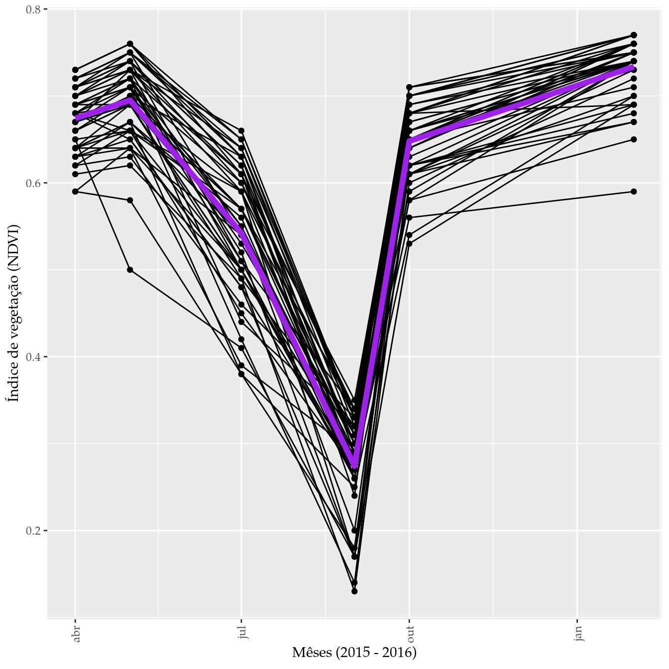
Teste da aditividade
## Analysis of Variance Table
##
## Response: ndvi
##              Df Sum Sq Mean Sq   F value    Pr(>F)
## factor(loc)  49 0.4375 0.00893    6.3517 < 2.2e-16 ***
## factor(mes)   5 7.1995 1.43991 1024.3405 < 2.2e-16 ***
## Residuals   245 0.3444 0.00141
## ---
## Signif. codes:  0 '***' 0.001 '**' 0.01 '*' 0.05 '.' 0.1 ' ' 1
# Verificação com o teste da não aditividade de Tukey.
with(teca_ndvi, {
agricolae::nonadditivity(y = ndvi,
factor1 = factor(loc),
factor2 = factor(mes),
df = df.residual(m0),
MSerror = deviance(m0)/df.residual(m0))
})##
## Tukey's test of nonadditivity
## ndvi
##
## P : -0.003201002
## Q : 0.04199744
##
## Analysis of Variance Table
##
## Response: residual
## Df Sum Sq Mean Sq F value Pr(>F)
## Nonadditivity 1 0.00024 0.00024398 0.173 0.6778
## Residuals 244 0.34415 0.00141045## $P
## Nonadditivity
## -0.003201002
##
## $Q
## Nonadditivity
## 0.04199744
##
## $ANOVA
## Analysis of Variance Table
##
## Response: residual
## Df Sum Sq Mean Sq F value Pr(>F)
## Nonadditivity 1 0.00024 0.00024398 0.173 0.6778
## Residuals 244 0.34415 0.00141045Regressão da produtividade pelo NDVI
# Médias de NDVI pra cada local.
teca_ndvim <- teca_ndvi %>%
    group_by(loc) %>%
    summarise(ndvi = mean(ndvi))

# Junção com valores de produção.
tb <- inner_join(teca_ndvim, teca_coords, by = "loc")
tb
## # A tibble: 50 x 6
## loc ndvi longitude latitude vol ima
## <int> <dbl> <dbl> <dbl> <dbl> <dbl>
## 1 1 0.558 333033. 8249775. 0.27 10.0
## 2 2 0.563 333663. 8249145. 0.1 3.57
## 3 3 0.565 333783. 8248845. 0.5 18.4
## 4 4 0.598 334893. 8249025. 0.41 15.1
## 5 5 0.618 335343. 8247765. 0.22 8.02
## 6 6 0.588 335253. 8248725. 0.09 3.22
## 7 7 0.6 335733. 8248395. 0.08 3.07
## 8 8 0.507 335433. 8249925. 0.41 15.0
## 9 9 0.562 336363. 8249205. 0.14 5.28
## 10 10 0.617 336603. 8249385. 0.18 6.53
## # … with 40 more rows# Relação de volume com IMA.
ggplot(data = tb,
mapping = aes(x = ima, y = vol)) +
geom_point() +
geom_smooth(method = "lm", color = "purple")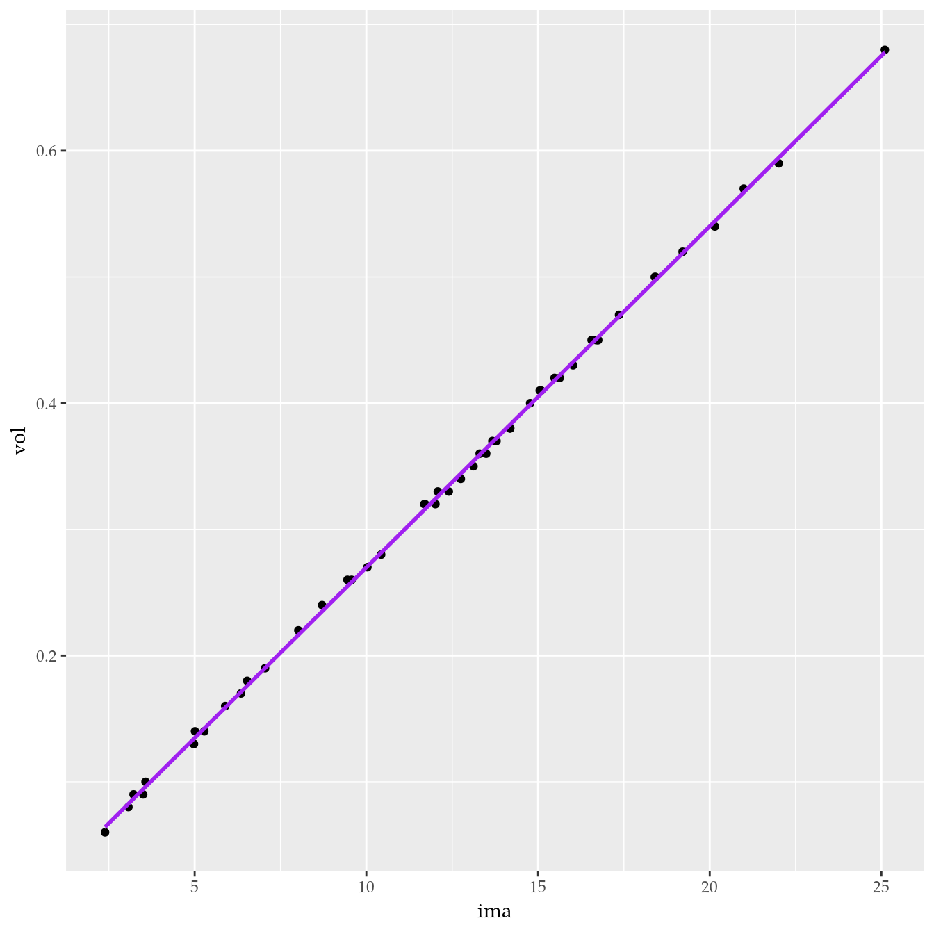
# Relação de volume com NDVI.
ggplot(data = tb,
       mapping = aes(x = ndvi, y = vol)) +
    geom_point() +
    geom_smooth(method = "lm", color = "purple")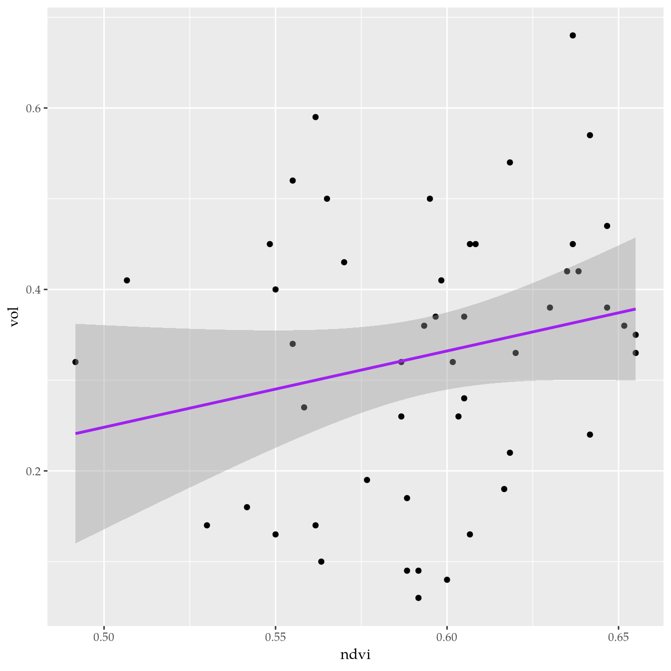
##
## Call:
## lm(formula = vol ~ ndvi, data = tb)
##
## Residuals:
##      Min       1Q   Median       3Q      Max
## -0.26519 -0.12621  0.00379  0.10702  0.31697
##
## Coefficients:
##             Estimate Std. Error t value Pr(>|t|)
## (Intercept)  -0.1723     0.3270  -0.527    0.601
## ndvi          0.8408     0.5488   1.532    0.132
##
## Residual standard error: 0.1482 on 48 degrees of freedom
## Multiple R-squared:  0.04662,    Adjusted R-squared:  0.02676
## F-statistic: 2.347 on 1 and 48 DF,  p-value: 0.1321
layout(1)Relação do NDVI com variáveis de solo
# Variáveis de solo.
teca_soil <- full_join(teca_qui, teca_crapar)
## Joining, by = c("loc", "cam")glimpse(teca_soil)## Observations: 150
## Variables: 23
## $ loc <int> 1, 1, 1, 2, 2, 2, 3, 3, 3, 4, 4, 4, 5, 5, 5, 6, 6, 6,…
## $ cam <fct> "[0, 5)", "[5, 40)", "[40, 80)", "[0, 5)", "[5, 40)",…
## $ ph <dbl> 6.8, 6.7, 6.7, 4.7, 4.7, 4.9, 7.6, 6.8, 6.9, 6.6, 6.2…
## $ p <dbl> 22.51, 0.83, 0.01, 3.89, 0.69, 0.10, 11.52, 1.66, 0.4…
## $ k <dbl> 72.24, 13.42, 7.23, 48.13, 12.34, 8.64, 114.55, 25.80…
## $ ca <dbl> 8.27, 2.91, 2.33, 0.97, 0.76, 0.21, 7.63, 3.22, 2.22,…
## $ mg <dbl> 1.70, 1.77, 0.51, 0.16, 0.14, 0.00, 1.53, 1.31, 1.09,…
## $ al <dbl> 0.0, 0.0, 0.0, 0.3, 0.6, 0.6, 0.0, 0.0, 0.0, 0.0, 0.0…
## $ ctc <dbl> 12.47, 6.57, 4.52, 5.30, 4.17, 3.47, 12.41, 6.26, 5.0…
## $ sat <dbl> 81.41, 71.74, 63.23, 23.66, 22.35, 6.69, 76.14, 73.44…
## $ mo <dbl> 72.2, 25.6, 9.7, 34.4, 8.7, 9.7, 50.4, 15.6, 9.5, 50.…
## $ arg <dbl> 183.7, 215.0, 285.5, 231.9, 212.6, 237.0, 192.6, 234.…
## $ are <dbl> 769.5, 749.5, 674.5, 741.0, 775.0, 752.0, 715.5, 698.…
## $ cas <dbl> 1.8, 2.2, 3.7, 0.4, 1.1, 1.7, 8.4, 19.0, 14.3, 5.5, 3…
## $ acc <dbl> 769.93, 750.04, 675.69, 741.11, 775.25, 752.42, 717.8…
## $ Ur <dbl> 0.22288275, 0.17845472, 0.18791987, 0.13107692, 0.164…
## $ Us <dbl> 0.6477212, 0.5799842, 0.6472682, 0.6967997, 0.5728316…
## $ alp <dbl> -0.7242483, -0.8327602, -0.7221707, -0.5484938, -0.54…
## $ n <dbl> 3.589612, 3.112403, 3.250733, 4.006821, 2.917137, 2.1…
## $ I <dbl> 0.8152153, 0.9572842, 0.8352604, 0.6201503, 0.6909264…
## $ Ui <dbl> 0.4497358, 0.3956184, 0.4353160, 0.4306964, 0.3870457…
## $ S <dbl> -0.34126593, -0.27326860, -0.32901803, -0.51467615, -…
## $ cad <dbl> 0.2268530, 0.2171637, 0.2473961, 0.2996195, 0.2221090…# Determinar valores médio a longo das 3 camadas.
teca_soil <- full_join(teca_qui, teca_crapar) %>%
group_by(loc) %>%
summarise_at(.vars = vars(ph:cad),
.funs = "mean")## Joining, by = c("loc", "cam")# Junta com valores de NDVI.
teca_soil <- inner_join(teca_soil, teca_ndvim)## Joining, by = "loc"glimpse(teca_soil)## Observations: 50
## Variables: 23
## $ loc <int> 1, 2, 3, 4, 5, 6, 7, 8, 9, 10, 11, 12, 13, 14, 15, 1…
## $ ph <dbl> 6.733333, 4.766667, 7.100000, 5.933333, 5.633333, 5.…
## $ p <dbl> 7.7833333, 1.5600000, 4.5300000, 9.2666667, 1.430000…
## $ k <dbl> 30.96333, 23.03667, 55.72667, 26.32333, 30.85000, 33…
## $ ca <dbl> 4.5033333, 0.6466667, 4.3566667, 2.8466667, 1.646666…
## $ mg <dbl> 1.3266667, 0.1000000, 1.3100000, 0.7133333, 0.893333…
## $ al <dbl> 0.00000000, 0.50000000, 0.00000000, 0.13333333, 0.13…
## $ ctc <dbl> 7.853333, 4.313333, 7.910000, 5.950000, 5.013333, 5.…
## $ sat <dbl> 72.12667, 17.56667, 72.12000, 52.95667, 45.80000, 28…
## $ mo <dbl> 35.83333, 17.60000, 25.16667, 22.80000, 19.86667, 16…
## $ arg <dbl> 228.0667, 227.1667, 217.5667, 189.9000, 330.3000, 29…
## $ are <dbl> 731.1667, 756.0000, 696.1667, 750.5000, 637.1667, 63…
## $ cas <dbl> 2.566667, 1.066667, 13.900000, 6.600000, 7.400000, 2…
## $ acc <dbl> 731.8867, 756.2600, 700.4267, 752.3133, 640.0000, 64…
## $ Ur <dbl> 0.1964191, 0.1560172, 0.3171179, 0.1762473, 0.178900…
## $ Us <dbl> 0.6249912, 0.6409684, 0.6734131, 0.5642064, 0.696111…
## $ alp <dbl> -0.75972639, -0.52218142, -0.75848102, -0.24335142, …
## $ n <dbl> 3.317583, 3.016808, 2.640506, 2.264469, 2.697576, 2.…
## $ I <dbl> 0.86925329, 0.69363093, 0.97993896, 0.56249512, 0.71…
## $ Ui <dbl> 0.4268901, 0.4213934, 0.5146961, 0.3963516, 0.466104…
## $ S <dbl> -0.3145175, -0.3245622, -0.2039071, -0.1837534, -0.2…
## $ cad <dbl> 0.2304710, 0.2653762, 0.1975782, 0.2201043, 0.287203…
## $ ndvi <dbl> 0.5583333, 0.5633333, 0.5650000, 0.5983333, 0.618333…# Empilha os valores das variáveis de solo.
tb <- teca_soil %>%
gather(key = "variable", value = "valor", ph:cad)
# Detemrina a média de NDVI para exibir no gráfico.
m <- mean(teca_soil$ndvi)
# Todas as variáveis.
ggplot(data = tb,
mapping = aes(x = valor, y = ndvi)) +
facet_wrap(facets = ~variable, scales = "free_x") +
geom_point() +
geom_smooth(method = "lm", se = TRUE) +
geom_hline(yintercept = m, linetype = 2, color = "red")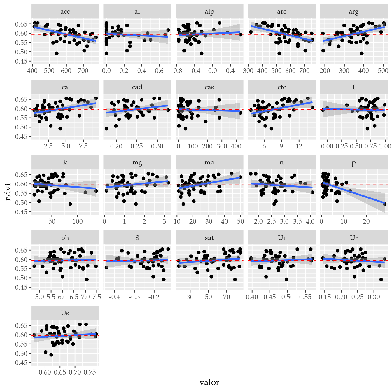
# Seleciona as variáveis com maior efeito.
tb_sel <- tb %>%
    filter(variable %in% c("acc", "are", "arg", "ctc", "mo", "ca", "cad"))

# Conjunto selecionado.
ggplot(data = tb_sel,
       mapping = aes(x = valor, y = ndvi)) +
    facet_wrap(facets = ~variable, scales = "free_x") +
    geom_point() +
    geom_smooth(method = "lm", se = TRUE) +
    geom_hline(yintercept = m, linetype = 2, color = "red")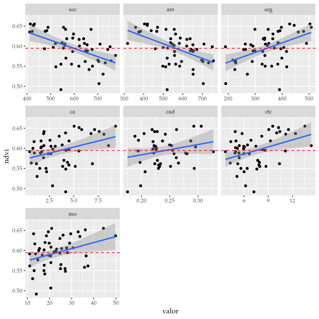
Informações da Sessão
## Atualizado em 11 de julho de 2019.
##
## R version 3.6.1 (2019-07-05)
## Platform: x86_64-pc-linux-gnu (64-bit)
## Running under: Ubuntu 18.04.2 LTS
##
## Matrix products: default
## BLAS:   /usr/lib/x86_64-linux-gnu/blas/libblas.so.3.7.1
## LAPACK: /usr/lib/x86_64-linux-gnu/lapack/liblapack.so.3.7.1
##
## locale:
##  [1] LC_CTYPE=pt_BR.UTF-8       LC_NUMERIC=C
##  [3] LC_TIME=pt_BR.UTF-8        LC_COLLATE=en_US.UTF-8
##  [5] LC_MONETARY=pt_BR.UTF-8    LC_MESSAGES=en_US.UTF-8
##  [7] LC_PAPER=pt_BR.UTF-8       LC_NAME=C
##  [9] LC_ADDRESS=C               LC_TELEPHONE=C
## [11] LC_MEASUREMENT=pt_BR.UTF-8 LC_IDENTIFICATION=C
##
## attached base packages:
## [1] stats     graphics  grDevices utils     datasets  methods
## [7] base
##
## other attached packages:
##  [1] forcats_0.4.0       stringr_1.4.0       dplyr_0.8.3
##  [4] purrr_0.3.2         readr_1.3.1         tidyr_0.8.3
##  [7] tibble_2.1.3        ggplot2_3.2.0       tidyverse_1.2.1
## [10] EACS_0.0-7          wzRfun_0.91         captioner_2.2.3
## [13] latticeExtra_0.6-28 RColorBrewer_1.1-2  lattice_0.20-38
## [16] knitr_1.23
##
## loaded via a namespace (and not attached):
##   [1] colorspace_1.4-1   deldir_0.1-22      class_7.3-15
##   [4] rprojroot_1.3-2    fs_1.3.1           rstudioapi_0.10
##   [7] roxygen2_6.1.1     remotes_2.1.0      fansi_0.4.0
##  [10] lubridate_1.7.4    xml2_1.2.0         splines_3.6.1
##  [13] pkgload_1.0.2      zeallot_0.1.0      jsonlite_1.6
##  [16] broom_0.5.2        cluster_2.1.0      shiny_1.3.2
##  [19] compiler_3.6.1     httr_1.4.0         backports_1.1.4
##  [22] assertthat_0.2.1   Matrix_1.2-17      lazyeval_0.2.2
##  [25] cli_1.1.0          later_0.8.0        htmltools_0.3.6
##  [28] prettyunits_1.0.2  tools_3.6.1        coda_0.19-3
##  [31] gtable_0.3.0       agricolae_1.3-1    glue_1.3.1
##  [34] gmodels_2.18.1     Rcpp_1.0.1         cellranger_1.1.0
##  [37] pkgdown_1.3.0      vctrs_0.2.0        spdep_1.1-2
##  [40] gdata_2.18.0       nlme_3.1-140       xfun_0.8
##  [43] ps_1.3.0           testthat_2.1.1     rvest_0.3.4
##  [46] mime_0.7           miniUI_0.1.1.1     gtools_3.8.1
##  [49] devtools_2.1.0     LearnBayes_2.15.1  MASS_7.3-51.4
##  [52] scales_1.0.0       hms_0.5.0          promises_1.0.1
##  [55] expm_0.999-4       yaml_2.2.0         memoise_1.1.0
##  [58] stringi_1.4.3      AlgDesign_1.1-7.3  highr_0.8
##  [61] klaR_0.6-14        desc_1.2.0         e1071_1.7-2
##  [64] boot_1.3-23        pkgbuild_1.0.3     spData_0.3.0
##  [67] rlang_0.4.0        pkgconfig_2.0.2    commonmark_1.7
##  [70] evaluate_0.14      sf_0.7-6           labeling_0.3
##  [73] processx_3.4.0     tidyselect_0.2.5   magrittr_1.5
##  [76] R6_2.4.0           generics_0.0.2     combinat_0.0-8
##  [79] DBI_1.0.0          pillar_1.4.2       haven_2.1.1
##  [82] withr_2.1.2        units_0.6-3        sp_1.3-1
##  [85] modelr_0.1.4       crayon_1.3.4       questionr_0.7.0
##  [88] utf8_1.1.4         KernSmooth_2.23-15 rmarkdown_1.13
##  [91] usethis_1.5.1      grid_3.6.1         readxl_1.3.1
##  [94] callr_3.3.0        digest_0.6.20      classInt_0.3-3
##  [97] xtable_1.8-4       httpuv_1.5.1       munsell_0.5.0
## [100] sessioninfo_1.1.1