Funções de pedotransferência para latossolos de Goiás
Walmes Marques Zeviani, Josué Gomes Delmond, Eduardo da Costa Severiano & Carla Eloize Carducci
11 de julho de 2019
Source:vignettes/pedotrans.Rmd
pedotrans.RmdAjuste da curva de retenção de água do solo
Ajuste por unidade experimental
## List of 3
##  $ pcc:'data.frame': 360 obs. of  7 variables:
##   ..$ unid: int [1:360] 1 1 1 1 1 1 1 1 1 1 ...
##   ..$ rept: int [1:360] 1 1 1 1 1 1 1 1 1 2 ...
##   ..$ tens: int [1:360] 0 1 2 6 10 33 100 1500 10000 0 ...
##   ..$ ppc : num [1:360] NA 135 127 137 220 ...
##   ..$ umid: num [1:360] 0.485 0.379 0.313 0.168 0.121 0.107 0.084 0.068 0.045 0.495 ...
##   ..$ ds  : num [1:360] NA 1.34 1.38 1.46 1.36 ...
##   ..$ co  : num [1:360] NA 3.5 3.2 3.6 3.3 3.1 3.1 3.3 3.2 NA ...
##  $ tex:'data.frame': 30 obs. of  6 variables:
##   ..$ unid  : int [1:30] 1 1 1 2 2 2 3 3 3 4 ...
##   ..$ metodo: Factor w/ 3 levels "Boy","Pip","Ultsom": 1 2 3 1 2 3 1 2 3 1 ...
##   ..$ arg   : num [1:30] 163 152 167 178 203 ...
##   ..$ sil   : num [1:30] 20 25 10 35 41.8 ...
##   ..$ are   : num [1:30] 817 823 823 787 756 ...
##   ..$ argsil: num [1:30] 183 177 177 213 244 ...
##  $ qui:'data.frame': 10 obs. of  5 variables:
##   ..$ unid : int [1:10] 1 2 3 4 5 6 7 8 9 10
##   ..$ silic: int [1:10] 24 34 24 62 92 41 56 90 87 180
##   ..$ alumi: int [1:10] 67 85 113 147 213 173 204 179 205 344
##   ..$ ferro: int [1:10] 38 85 116 68 78 177 231 298 245 105
##   ..$ dp   : num [1:10] 2.66 2.76 2.75 2.76 2.67 2.81 2.95 2.92 2.92 2.69
# Valores relacionados à tensão.
pdt <- pedotrans$pcc
# Troca tensão 0 por algo positivo para não desaparecer com o log.
pdt$tens[pdt$tens == 0] <- 0.1
pdt$ltens <- log(pdt$tens)
# Cria unidade experimental.
pdt$ue <- with(pdt, interaction(unid, rept, drop = FALSE))
# Para mudar a ordem dos níveis.
l <- c(t(matrix(levels(pdt$ue), nrow = 10)))
pdt$ue <- factor(pdt$ue, levels = l)
str(pdt)## 'data.frame': 360 obs. of 9 variables:
## $ unid : int 1 1 1 1 1 1 1 1 1 1 ...
## $ rept : int 1 1 1 1 1 1 1 1 1 2 ...
## $ tens : num 0.1 1 2 6 10 33 100 1500 10000 0.1 ...
## $ ppc : num NA 135 127 137 220 ...
## $ umid : num 0.485 0.379 0.313 0.168 0.121 0.107 0.084 0.068 0.045 0.495 ...
## $ ds : num NA 1.34 1.38 1.46 1.36 ...
## $ co : num NA 3.5 3.2 3.6 3.3 3.1 3.1 3.3 3.2 NA ...
## $ ltens: num -2.303 0 0.693 1.792 2.303 ...
## $ ue : Factor w/ 40 levels "1.1","1.2","1.3",..: 1 1 1 1 1 1 1 1 1 2 ...## Using umid as value column: use value.var to override.## tens 1 2 3 4
## 1 0.1 0.485 0.495 0.482 0.494
## 2 1.0 0.379 0.390 0.350 0.386
## 3 2.0 0.313 0.329 0.323 0.332
## 4 6.0 0.168 0.161 0.161 0.163
## 5 10.0 0.121 0.116 0.125 0.112
## 6 33.0 0.107 0.103 0.103 0.101
## 7 100.0 0.084 0.081 0.093 0.091
## 8 1500.0 0.068 0.066 0.068 0.053
## 9 10000.0 0.045 0.046 0.044 0.047xyplot(umid ~ tens | as.factor(unid),
groups = rept,
data = pdt,
jitter.x = TRUE,
type = c("p", "a"),
as.table = TRUE,
xscale.components = xscale.components.logpower,
xlab = "Logaritmo base 10 da tensão aplicada (kPa)",
ylab = expression("Umidade do solo" ~ (dm^{3} ~ dm^{-3})),
scales = list(x = list(log = 10)))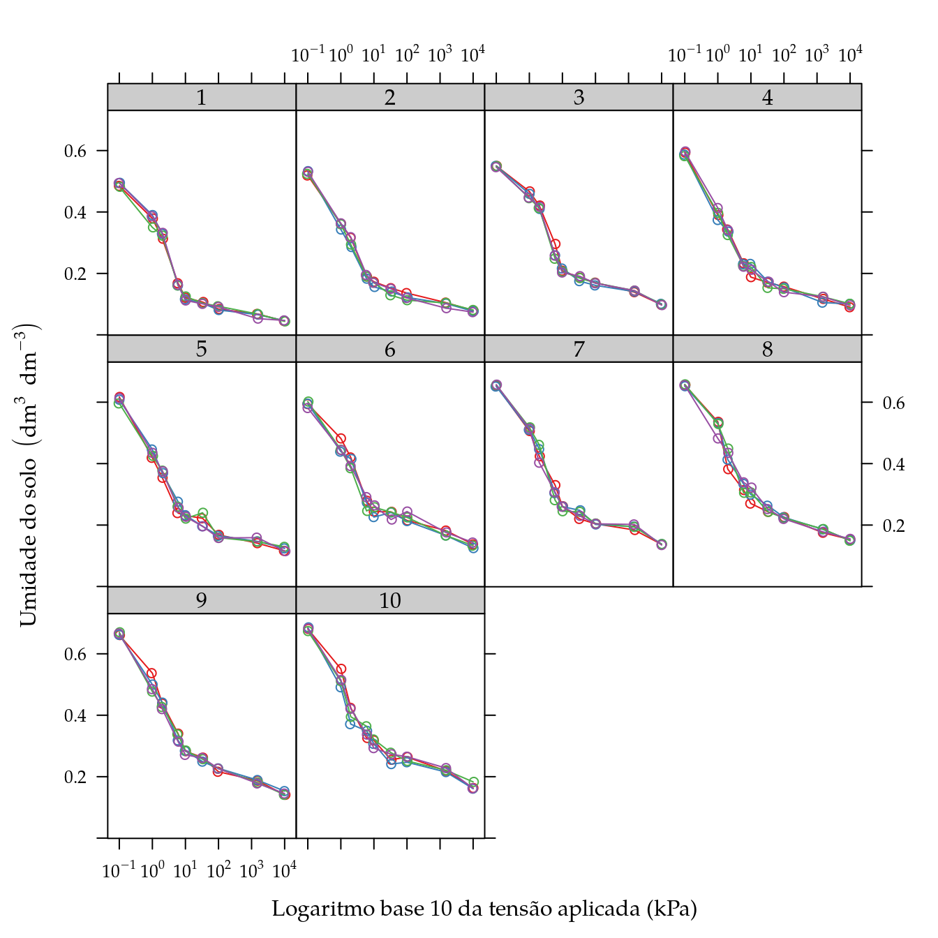
# Ajuste com interface gráfica para posicionar a curva e ter
# convergência certa.

library(rpanel)

fit <- rp.nls(
    model = umid ~ thr + (ths - thr)/(1 + exp(tha + ltens)^thn)^(1 - 1/thn),
    data = pdt,
    start = list(thr = c(0, 0.2, 0.5),
                 ths = c(0.5, 1, 0.7),
                 tha = c(-3, 3, 1),
                 thn = c(1.1, 1.8, 1.5)),
    subset = "ue")

dput(sapply(fit, function(x) round(coef(x), 4)))
estimates <-
structure(c(0.061, 0.4855, -0.118, 1.7796, 0.0928, 0.5308, 0.6793,
1.5288, 0.1197, 0.5503, -0.2914, 1.6156, 0.0988, 0.6186, 1.1132,
1.4495, 0.1222, 0.6502, 1.3007, 1.42, 0.1659, 0.601, 0.203, 1.5824,
0.1533, 0.6647, 0.4815, 1.4977, 0.1708, 0.6708, 0.4919, 1.5473,
0.1556, 0.6746, 0.494, 1.4457, 0.1937, 0.6966, 0.587, 1.5036,
0.0615, 0.4923, -0.2585, 1.8835, 0.0895, 0.5511, 0.9341, 1.5466,
0.1233, 0.5502, -0.2379, 1.678, 0.0859, 0.6408, 1.7727, 1.3445,
0.1287, 0.622, 0.6943, 1.4923, 0.1427, 0.6097, 0.7708, 1.4351,
0.1645, 0.6588, 0.3134, 1.5514, 0.1586, 0.6694, 0.6833, 1.415,
0.1638, 0.6775, 0.7306, 1.4431, 0.1713, 0.7435, 1.7755, 1.355,
0.0588, 0.4813, 0.0365, 1.6922, 0.0895, 0.5349, 0.6368, 1.5824,
0.1268, 0.5484, -0.1657, 1.6755, 0.1072, 0.6024, 0.9629, 1.4858,
0.13, 0.6146, 0.9213, 1.4441, 0.1502, 0.6244, 1.0353, 1.4251,
0.1727, 0.6586, 0.052, 1.7006, 0.1649, 0.6689, 0.3891, 1.4947,
0.1331, 0.7121, 1.5491, 1.3126, 0.1844, 0.712, 1.464, 1.3515,
0.0589, 0.4909, -0.2484, 1.8562, 0.0773, 0.5457, 0.786, 1.484,
0.1252, 0.5455, -0.2012, 1.6576, 0.1058, 0.6144, 0.8225, 1.5077,
0.1302, 0.6269, 0.7135, 1.5172, 0.1543, 0.5982, 0.9032, 1.4007,
0.1677, 0.6684, 0.4493, 1.5709, 0.1362, 0.6839, 1.2749, 1.3142,
0.1498, 0.6949, 1.1838, 1.3787, 0.1901, 0.7087, 1.0781, 1.4224
), .Dim = c(4L, 40L), .Dimnames = list(c("thr", "ths", "tha",
"thn"), c("1.1", "2.1", "3.1", "4.1", "5.1", "6.1", "7.1", "8.1",
"9.1", "10.1", "1.2", "2.2", "3.2", "4.2", "5.2", "6.2", "7.2",
"8.2", "9.2", "10.2", "1.3", "2.3", "3.3", "4.3", "5.3", "6.3",
"7.3", "8.3", "9.3", "10.3", "1.4", "2.4", "3.4", "4.4", "5.4",
"6.4", "7.4", "8.4", "9.4", "10.4")))
#-----------------------------------------------------------------------
# Ajustar novamente para ter precisão cheia nas estimativas que foram
# arredondadas para salvar espaço e ter objetos `nls`.
f <- umid ~ thr + (ths - thr)/(1 + exp(tha + ltens)^thn)^(1 - 1/thn)
fit <- vector(mode = "list", length = nlevels(pdt$ue))
names(fit) <- levels(pdt$ue)
for (i in names(fit)) {
fit[[i]] <- nls(f,
data = subset(pdt, ue == i),
start = estimates[, i])
}
estimates <- sapply(fit, FUN = coef)
# Valores médios dos parâmetros.
rowMeans(estimates)## thr ths tha thn
## 0.1309244 0.6173387 0.6440523 1.5197176# Pares de diagramas de dispersão.
splom(t(estimates),
groups = sub("\\..*", "", colnames(estimates)),
as.matrix = TRUE)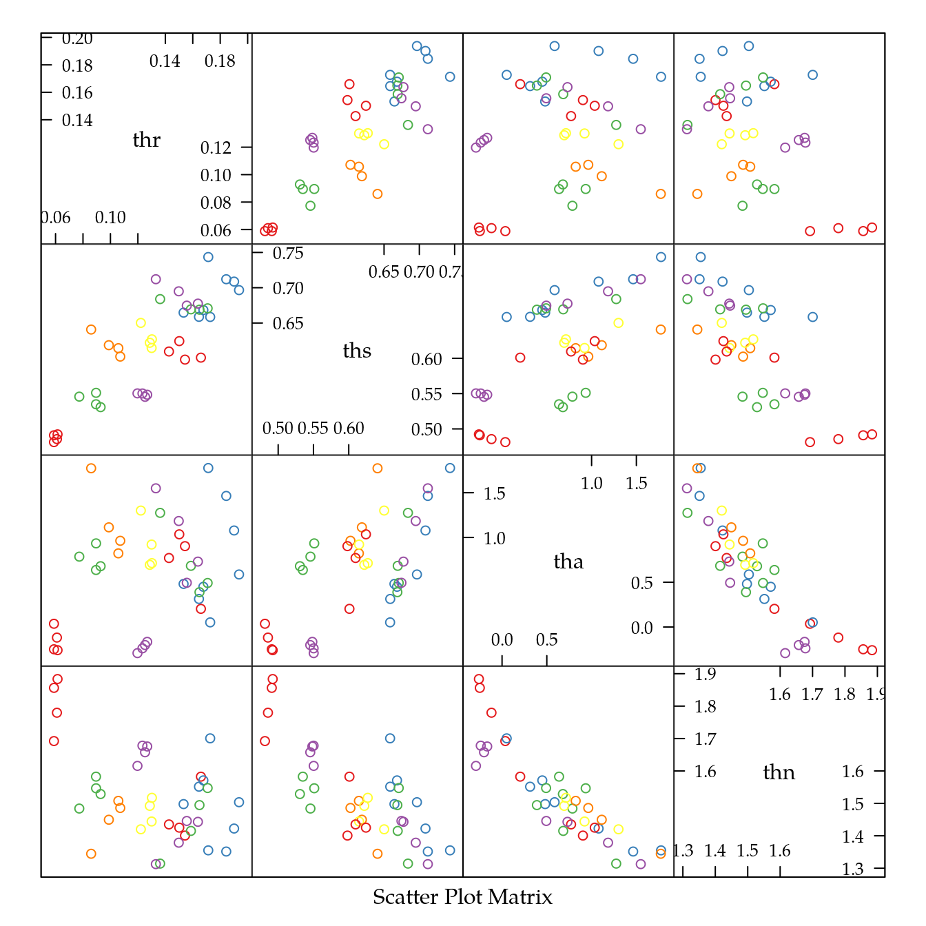
#-----------------------------------------------------------------------
# Ajuste com a nlsList() para ter os intervalos de confiança.

n0 <- nlsList(
    model = umid ~ thr + (ths - thr)/(1 + exp(tha + ltens)^thn)^(1 - 1/thn) | ue,
    data = subset(pdt, select = c(ltens, umid, ue)),
    start = rowMeans(estimates))

p <- plot(intervals(n0),
          layout = c(4, NA))
update(p,
       xlab = "Estimativa",
       ylab = "Unidade experimental")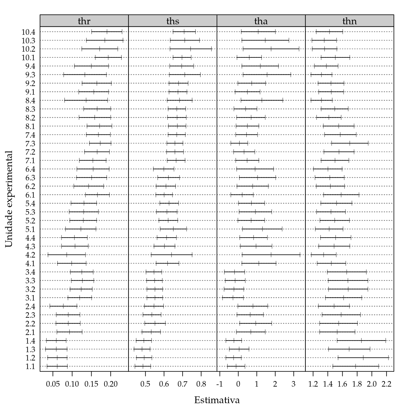
Índices S e I
#-----------------------------------------------------------------------
# Cálculo dos índices S e I.

# Transforma de matriz para tabela.
params <- cbind(as.data.frame(t(estimates)),
                ue = colnames(estimates))
rownames(params) <- NULL

# Adiciona as colunas de `unid` e `rept`.
params <- merge(unique(subset(pdt, select = c(unid, rept, ue))),
                params,
                by = "ue")

# Ordena pelos níveis de `ue`.
params <- params[order(params$ue), ]

# Calcula S e I.
params <- within(params, {
    S <- -(ths - thr) * thn * (1 + 1/(1 - 1/thn))^(-(1 - 1/thn) - 1)
    I <- -tha - log(1 - 1/thn)/thn
    U <- thr + (ths - thr)/(1 + exp(tha + I)^thn)^(1 - 1/thn)
})
str(params)
## 'data.frame': 40 obs. of 10 variables:
## $ ue : Factor w/ 40 levels "1.1","1.2","1.3",..: 1 2 3 4 5 6 7 8 9 10 ...
## $ unid: int 1 1 1 1 2 2 2 2 3 3 ...
## $ rept: int 1 2 3 4 1 2 3 4 1 2 ...
## $ thr : num 0.061 0.0615 0.0588 0.0589 0.0928 ...
## $ ths : num 0.486 0.492 0.481 0.491 0.531 ...
## $ tha : num -0.118 -0.2585 0.0365 -0.2484 0.6793 ...
## $ thn : num 1.78 1.88 1.69 1.86 1.53 ...
## $ U : num 0.313 0.314 0.314 0.313 0.367 ...
## $ I : num 0.5818 0.6604 0.4918 0.6653 0.0152 ...
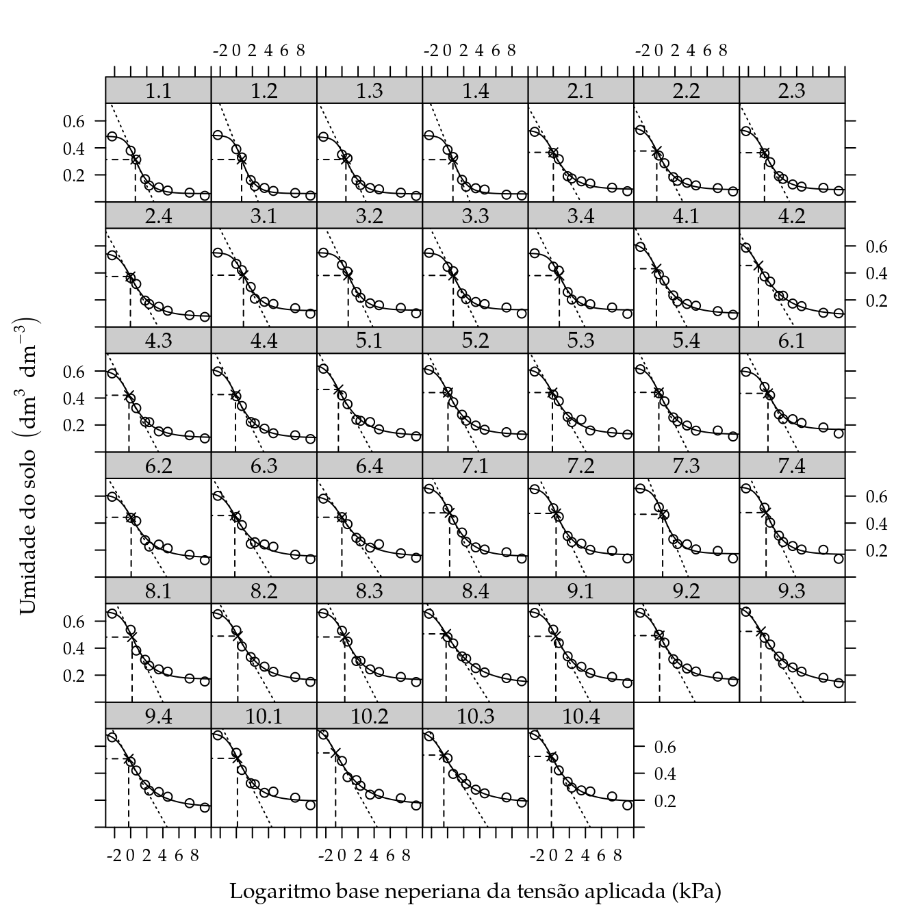
## $ S : num -0.137 -0.152 -0.125 -0.149 -0.108 ...xyplot(umid ~ ltens | as.factor(ue),
data = pdt,
as.table = TRUE,
xlab = "Logaritmo base neperiana da tensão aplicada (kPa)",
ylab = expression("Umidade do solo" ~ (dm^{3} ~ dm^{-3}))) +
layer({
p <- as.list(params[packet.number(), ])
with(p, {
# Curva ajustada.
panel.curve(
thr + (ths - thr)/(1 + exp(tha + x)^thn)^(1 - 1/thn))
# Tensão, umidade e inclinação no ponto de inflexão.
panel.points(x = I, y = U, pch = 4)
panel.segments(I, 0, I, U, lty = 2)
panel.segments(-5, U, I, U, lty = 2)
panel.abline(a = U - S * I, b = S, lty = 3)
})
})
Valores médios dos parâmetros por local
#-----------------------------------------------------------------------
# Valores médios dos parâmetros para cada unidade de latossolo.

# Valores para os parâmetros da CRAS.
crap <- summarise_all(
    .tbl = group_by(.data = subset(params, select = -c(ue, rept)),
                    unid),
    .funs = funs(mean))

# round(as.data.frame(crap), 4)
round(crap, digits = 4)
## # A tibble: 10 x 8
## unid thr ths tha thn U I S
## <dbl> <dbl> <dbl> <dbl> <dbl> <dbl> <dbl> <dbl>
## 1 1 0.06 0.488 -0.147 1.80 0.313 0.600 -0.141
## 2 2 0.0873 0.541 0.759 1.54 0.370 -0.0706 -0.112
## 3 3 0.124 0.549 -0.224 1.66 0.382 0.783 -0.121
## 4 4 0.0994 0.619 1.17 1.45 0.433 -0.344 -0.113
## 5 5 0.128 0.628 0.907 1.47 0.446 -0.126 -0.113
## 6 6 0.153 0.608 0.728 1.46 0.444 0.0733 -0.101
## 7 7 0.165 0.663 0.324 1.58 0.472 0.318 -0.13
## 8 8 0.158 0.673 0.710 1.44 0.490 0.132 -0.111
## 9 9 0.151 0.690 0.989 1.40 0.503 -0.0738 -0.108
## 10 10 0.185 0.715 1.23 1.41 0.53 -0.335 -0.108Estudo de correlação com variáveis texturais
ATTENTION: qual dos métodos de determinação das variáveis texturais gera o conjunto de variáveis texturais com maior poder de explicação para as variáveis hídricas? Explorar a correlação canônica? Esse grau de explicação muda com o tipo de método?
# Junta variáveis hídricas com texturais.
cratex <- merge(crap, pedotrans$tex, by = "unid", all = TRUE)

# # Gráfico de pares de diagramas de dispersão.
# splom(subset(cratex, select = -c(unid, metodo)),
#       groups = cratex$metodo,
#       type = c("p", "r"))

cra <- names(crap)[-1]
tex <- names(pedotrans$tex)[-(1:2)]

# Correlações entre os conjuntos de variáveis separado por método.
b <- by(data = cratex,
        INDICES = cratex$metodo,
        FUN = function(x) {
            k <- cor(subset(x, select = -c(unid, metodo)),
                     method = "spearman")
            k <- k[cra, tex]
            m <- as.character(x$metodo[1])
            print(m)
            print(k)
            k <- cbind(stack(as.data.frame(k)), cra = rownames(k))
            names(k)[1:2] <- c(m, "tex")
            return(k)
        })
## [1] "Boy"
## arg sil are argsil
## thr 0.9030303 0.6606061 -0.8787879 0.8787879
## ths 0.9636364 0.7575758 -0.9878788 0.9878788
## tha 0.4909091 0.2606061 -0.5151515 0.5151515
## thn -0.8060606 -0.4787879 0.7939394 -0.7939394
## U 0.9878788 0.7818182 -1.0000000 1.0000000
## I -0.3696970 -0.2363636 0.4060606 -0.4060606
## S 0.6121212 0.2606061 -0.5393939 0.5393939
## [1] "Pip"
## arg sil are argsil
## thr 0.9030303 0.6484848 -0.8787879 0.8787879
## ths 0.9636364 0.7818182 -0.9878788 0.9878788
## tha 0.4909091 0.3575758 -0.5151515 0.5151515
## thn -0.8060606 -0.5393939 0.7939394 -0.7939394
## U 0.9878788 0.7939394 -1.0000000 1.0000000
## I -0.3696970 -0.3454545 0.4060606 -0.4060606
## S 0.6121212 0.2848485 -0.5393939 0.5393939
## [1] "Ultsom"
## arg sil are argsil
## thr 0.9030303 0.68484848 -0.8787879 0.8787879
## ths 0.9636364 0.74545455 -0.9878788 0.9878788
## tha 0.4909091 -0.05454545 -0.5151515 0.5151515
## thn -0.8060606 -0.28484848 0.7939394 -0.7939394
## U 0.9878788 0.73333333 -1.0000000 1.0000000
## I -0.3696970 0.12727273 0.4060606 -0.4060606
## S 0.6121212 -0.09090909 -0.5393939 0.5393939# Coloca as correlações lado a lado.
correl <- Reduce(
f = function(x, y) {
merge(x, y, by = c("tex", "cra"))
},
x = b)
m <- levels(pedotrans$tex$metodo)
# Número de vezes que cada método apresentou a maior correlação.
table(apply(correl[, m],
MARGIN = 1,
FUN = function(x) {
m[which.max(abs(x))]
}))##
## Boy Pip Ultsom
## 21 6 1Análise de correlação canônica
suppressPackageStartupMessages(library(candisc))

cc <- by(data = cratex,
         INDICES = cratex$metodo,
         FUN = function(x) {
             candisc::cancor(x = x[, c("arg", "sil")],
                             y = x[, c("ths", "thr", "tha", "thn",
                                       "U", "S", "I")])
        })

# Resumo do ajuste.
cc
## cratex$metodo: Boy
##
## Canonical correlation analysis of:
## 2 X variables: arg, sil
## with 7 Y variables: ths, thr, tha, thn, U, S, I
##
## CanR CanRSQ Eigen percent cum scree
## 1 0.9997 0.9994 1614.958 99.8459 99.85 ******************************
## 2 0.8448 0.7137 2.493 0.1541 100.00
##
## Test of H0: The canonical correlations in the
## current row and all that follow are zero
##
## CanR LR test stat approx F numDF denDF Pr(> F)
## 1 0.99969 0.000177 10.590 14 2 0.08953 .
## 2 0.84481 0.286293 0.831 6 2 0.63645
## ---
## Signif. codes: 0 '***' 0.001 '**' 0.01 '*' 0.05 '.' 0.1 ' ' 1
## ------------------------------------------------------------
## cratex$metodo: Pip
##
## Canonical correlation analysis of:
## 2 X variables: arg, sil
## with 7 Y variables: ths, thr, tha, thn, U, S, I
##
## CanR CanRSQ Eigen percent cum scree
## 1 0.9981 0.9963 268.537 99.2308 99.23 ******************************
## 2 0.8219 0.6755 2.082 0.7692 100.00
##
## Test of H0: The canonical correlations in the
## current row and all that follow are zero
##
## CanR LR test stat approx F numDF denDF Pr(> F)
## 1 0.99814 0.0012 3.9744 14 2 0.2190
## 2 0.82189 0.3245 0.6939 6 2 0.6918
## ------------------------------------------------------------
## cratex$metodo: Ultsom
##
## Canonical correlation analysis of:
## 2 X variables: arg, sil
## with 7 Y variables: ths, thr, tha, thn, U, S, I
##
## CanR CanRSQ Eigen percent cum scree
## 1 0.9963 0.9925 133.112 95.347 95.35 ******************************
## 2 0.9309 0.8666 6.496 4.653 100.00 *
##
## Test of H0: The canonical correlations in the
## current row and all that follow are zero
##
## CanR LR test stat approx F numDF denDF Pr(> F)
## 1 0.99626 0.000995 4.3868 14 2 0.2009
## 2 0.93092 0.133396 2.1655 6 2 0.3492par(mfrow = c(2, 2))
# heplot(cc[[1]], which = c(1, 2))
# heplot(cc[[2]], which = c(1, 2))
# heplot(cc[[3]], which = c(1, 2))
invisible(lapply(cc, FUN = heplot, which = c(1, 2)))## Vector scale factor set to 1## Vector scale factor set to 1## Vector scale factor set to 1layout(1)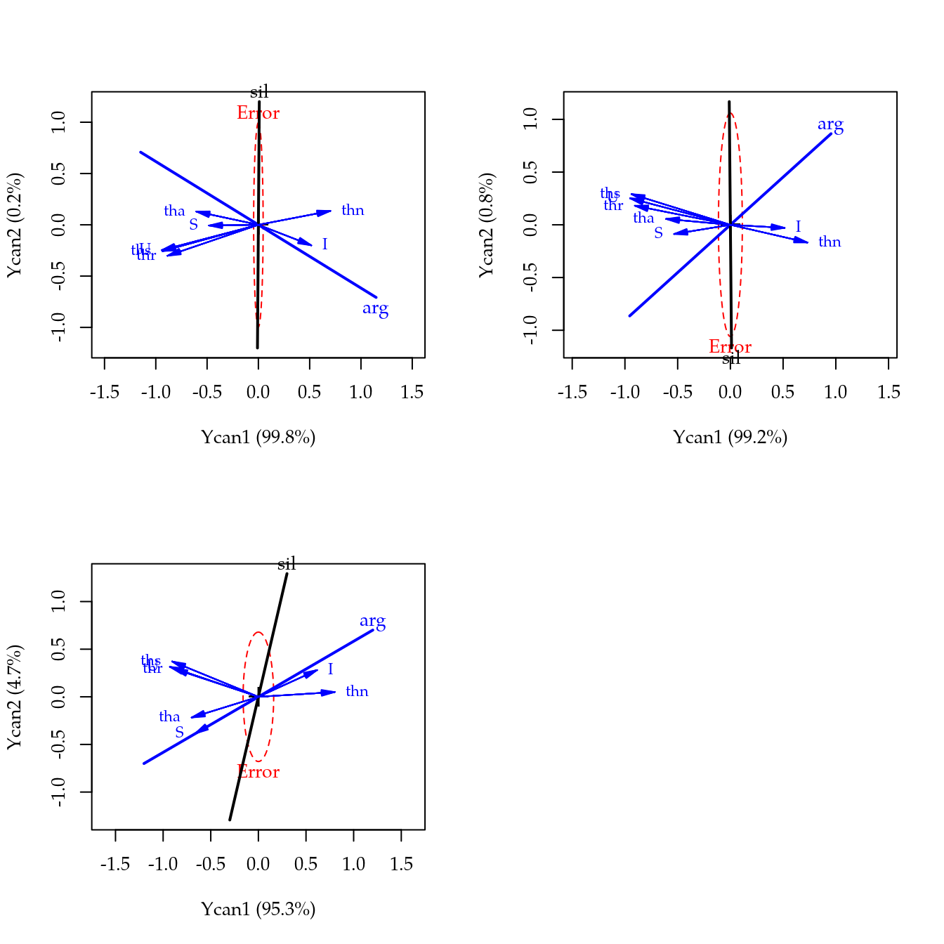
Ajuste da curva de pressão de preconsolidação
xyplot(ppc ~ tens | as.factor(unid),
       groups = rept,
       data = pedotrans$pcc,
       jitter.x = TRUE,
       type = c("p", "a"),
       as.table = TRUE,
       xscale.components = xscale.components.logpower,
       xlab = "Logaritmo base 10 da tensão aplicada (kPa)",
       ylab = "Pressão de preconsolidação (kPa)",
       scales = list(x = list(log = 10)))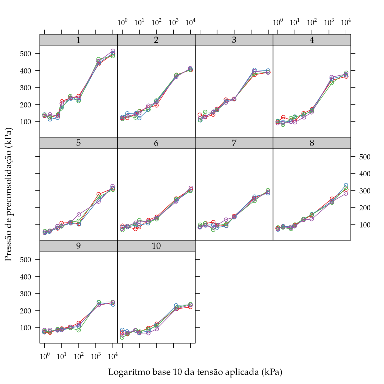
Informações da sessão
## Atualizado em 11 de julho de 2019.
##
## R version 3.6.1 (2019-07-05)
## Platform: x86_64-pc-linux-gnu (64-bit)
## Running under: Ubuntu 18.04.2 LTS
##
## Matrix products: default
## BLAS:   /usr/lib/x86_64-linux-gnu/blas/libblas.so.3.7.1
## LAPACK: /usr/lib/x86_64-linux-gnu/lapack/liblapack.so.3.7.1
##
## locale:
##  [1] LC_CTYPE=pt_BR.UTF-8       LC_NUMERIC=C
##  [3] LC_TIME=pt_BR.UTF-8        LC_COLLATE=en_US.UTF-8
##  [5] LC_MONETARY=pt_BR.UTF-8    LC_MESSAGES=en_US.UTF-8
##  [7] LC_PAPER=pt_BR.UTF-8       LC_NAME=C
##  [9] LC_ADDRESS=C               LC_TELEPHONE=C
## [11] LC_MEASUREMENT=pt_BR.UTF-8 LC_IDENTIFICATION=C
##
## attached base packages:
## [1] stats     graphics  grDevices utils     datasets  methods   base
##
## other attached packages:
##  [1] candisc_0.8-0       heplots_1.3-5       car_3.0-3
##  [4] carData_3.0-2       EACS_0.0-7          nlme_3.1-140
##  [7] dplyr_0.8.3         reshape2_1.4.3      wzRfun_0.91
## [10] captioner_2.2.3     latticeExtra_0.6-28 RColorBrewer_1.1-2
## [13] lattice_0.20-38     knitr_1.23
##
## loaded via a namespace (and not attached):
##  [1] Rcpp_1.0.1        prettyunits_1.0.2 ps_1.3.0          assertthat_0.2.1
##  [5] zeallot_0.1.0     rprojroot_1.3-2   digest_0.6.20     utf8_1.1.4
##  [9] cellranger_1.1.0  R6_2.4.0          plyr_1.8.4        backports_1.1.4
## [13] evaluate_0.14     pillar_1.4.2      rlang_0.4.0       readxl_1.3.1
## [17] curl_3.3          rstudioapi_0.10   data.table_1.12.2 callr_3.3.0
## [21] rmarkdown_1.13    pkgdown_1.3.0     desc_1.2.0        devtools_2.1.0
## [25] stringr_1.4.0     foreign_0.8-71    compiler_3.6.1    xfun_0.8
## [29] pkgconfig_2.0.2   pkgbuild_1.0.3    htmltools_0.3.6   tidyselect_0.2.5
## [33] tibble_2.1.3      roxygen2_6.1.1    rio_0.5.16        fansi_0.4.0
## [37] crayon_1.3.4      withr_2.1.2       MASS_7.3-51.4     commonmark_1.7
## [41] grid_3.6.1        magrittr_1.5      zip_2.0.3         cli_1.1.0
## [45] stringi_1.4.3     fs_1.3.1          remotes_2.1.0     testthat_2.1.1
## [49] xml2_1.2.0        vctrs_0.2.0       openxlsx_4.1.0.1  forcats_0.4.0
## [53] tools_3.6.1       glue_1.3.1        purrr_0.3.2       hms_0.5.0
## [57] abind_1.4-5       processx_3.4.0    pkgload_1.0.2     yaml_2.2.0
## [61] sessioninfo_1.1.1 memoise_1.1.0     haven_2.1.1       usethis_1.5.1