Modelagem da capacidade de suporte de carga de latossolos com diferente mineralogia
Walmes Marques Zeviani & Carla Eloize Carducci
19 de julho de 2019
Source:vignettes/cafe_pedotrans.Rmd
cafe_pedotrans.RmdExploratory data analysis
#-----------------------------------------------------------------------
# Load packages.

rm(list = objects())

library(EACS)
library(lmerTest)
library(lme4)
library(emmeans)
library(car)
library(tidyverse)
# Dataset.
da <- as_tibble(cafe_pedotrans)
str(da)## Classes 'tbl_df', 'tbl' and 'data.frame': 180 obs. of 11 variables:
## $ solo : Factor w/ 2 levels "LVAd","LVd": 2 2 2 2 2 2 2 2 2 2 ...
## $ tensao: int 6 6 6 6 6 6 6 6 6 6 ...
## $ posi : Factor w/ 2 levels "Entrelinha","Linha": 1 1 1 1 1 1 1 1 1 2 ...
## $ prof : Factor w/ 3 levels "0.00-0.05 m",..: 1 1 1 2 2 2 3 3 3 1 ...
## $ rep : int 1 2 3 1 2 3 1 2 3 1 ...
## $ dsi : num 0.84 0.82 0.99 0.84 0.95 0.99 0.83 0.92 0.91 0.86 ...
## $ dsp : num 0.9 0.82 0.99 0.99 0.99 1.04 0.92 0.95 0.97 0.87 ...
## $ thetai: num 0.506 0.481 0.465 0.451 0.421 ...
## $ ppc : num 125.2 86.4 207.5 256.7 120.3 ...
## $ trt : Factor w/ 12 levels "LVAd_Entrelinha_0.00-0.05 m",..: 2 2 2 6 6 6 10 10 10 4 ...
## $ ue : Factor w/ 36 levels "LVAd_Entrelinha_0.00-0.05 m_1",..: 2 14 26 6 18 30 10 22 34 4 ...# Recode factor levels.
levels(da$posi) <- c("Interrow", "Row")
s <- c(KH = "Kaolinitic Haplustox", GA = "Gibbsitic Acrustox")
levels(da$solo) <- names(s)
levels(da$prof)## [1] "0.00-0.05 m" "0.10-0.15 m" "0.20-0.25 m"# Recode levels.
da$trt <- with(da, interaction(solo, posi, as.integer(prof), sep = "·"))
# Numeric summary.
summary(da)## solo tensao posi prof
## KH:90 Min. : 6.0 Interrow:90 0.00-0.05 m:60
## GA:90 1st Qu.: 33.0 Row :90 0.10-0.15 m:60
## Median : 100.0 0.20-0.25 m:60
## Mean : 927.8
## 3rd Qu.:1500.0
## Max. :3000.0
##
## rep dsi dsp thetai
## Min. :1 Min. :0.3300 Min. :0.810 Min. :0.0800
## 1st Qu.:1 1st Qu.:0.8700 1st Qu.:0.930 1st Qu.:0.2951
## Median :2 Median :0.9400 Median :0.990 Median :0.3498
## Mean :2 Mean :0.9418 Mean :1.008 Mean :0.3219
## 3rd Qu.:3 3rd Qu.:1.0000 3rd Qu.:1.080 3rd Qu.:0.3902
## Max. :3 Max. :1.1800 Max. :1.240 Max. :0.5064
##
## ppc trt
## Min. : 51.55 KH·Interrow·1:15
## 1st Qu.: 99.76 GA·Interrow·1:15
## Median :168.53 KH·Row·1 :15
## Mean :214.15 GA·Row·1 :15
## 3rd Qu.:319.83 KH·Interrow·2:15
## Max. :535.24 GA·Interrow·2:15
## (Other) :90
## ue
## LVAd_Entrelinha_0.00-0.05 m_1: 5
## LVd_Entrelinha_0.00-0.05 m_1 : 5
## LVAd_Linha_0.00-0.05 m_1 : 5
## LVd_Linha_0.00-0.05 m_1 : 5
## LVAd_Entrelinha_0.10-0.15 m_1: 5
## LVd_Entrelinha_0.10-0.15 m_1 : 5
## (Other) :150# Count of experimental points.
ftable(tensao ~ solo + posi + prof, data = da)## tensao 6 33 100 1500 3000
## solo posi prof
## KH Interrow 0.00-0.05 m 3 3 3 3 3
## 0.10-0.15 m 3 3 3 3 3
## 0.20-0.25 m 3 3 3 3 3
## Row 0.00-0.05 m 3 3 3 3 3
## 0.10-0.15 m 3 3 3 3 3
## 0.20-0.25 m 3 3 3 3 3
## GA Interrow 0.00-0.05 m 3 3 3 3 3
## 0.10-0.15 m 3 3 3 3 3
## 0.20-0.25 m 3 3 3 3 3
## Row 0.00-0.05 m 3 3 3 3 3
## 0.10-0.15 m 3 3 3 3 3
## 0.20-0.25 m 3 3 3 3 3# Creates variables in the log scale.
da$logtensao <- log10(da$tensao)
da$logppc <- log10(da$ppc)
# Text to be used as axis label.
axis_text <- list(
pcc = expression(Log[10] ~ (sigma * "p, kPa") - "Preconsolidation pressure"),
tensao = expression(Log[10] ~ (Psi * "m, kPa") - "Matric tension"),
posi = "Position",
solo = "Soil",
prof = "Depth")
# Experimental units profile in each experimental point.
ggplot(data = da,
mapping = aes(x = tensao, y = ppc, color = rep, group = rep)) +
facet_wrap(facets = ~trt) +
geom_point(show.legend = FALSE) +
geom_line(show.legend = FALSE) +
scale_x_log10() +
scale_y_log10() +
labs(x = axis_text$tensao,
y = axis_text$pcc)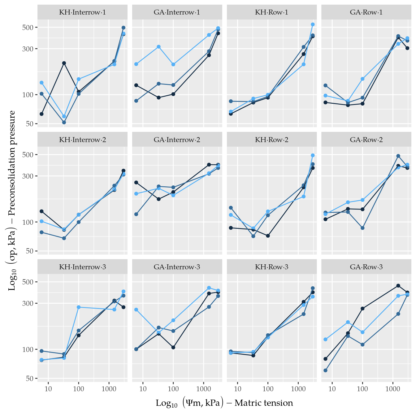
# Mean profile in each experimental point. The curve is the second order
# polynomial model fitted to the sample data only to check if it
# captures properly the trend in data.
ggplot(data = da,
       mapping = aes(x = tensao, y = ppc)) +
    facet_wrap(facets = ~trt) +
    geom_point() +
    stat_summary(geom = "line", fun.y = "mean") +
    geom_smooth(method = "lm",
                formula = y ~ poly(x, degree = 2),
                se = FALSE) +
    scale_x_log10() +
    scale_y_log10() +
    labs(x = axis_text$tensao,
         y = axis_text$pcc)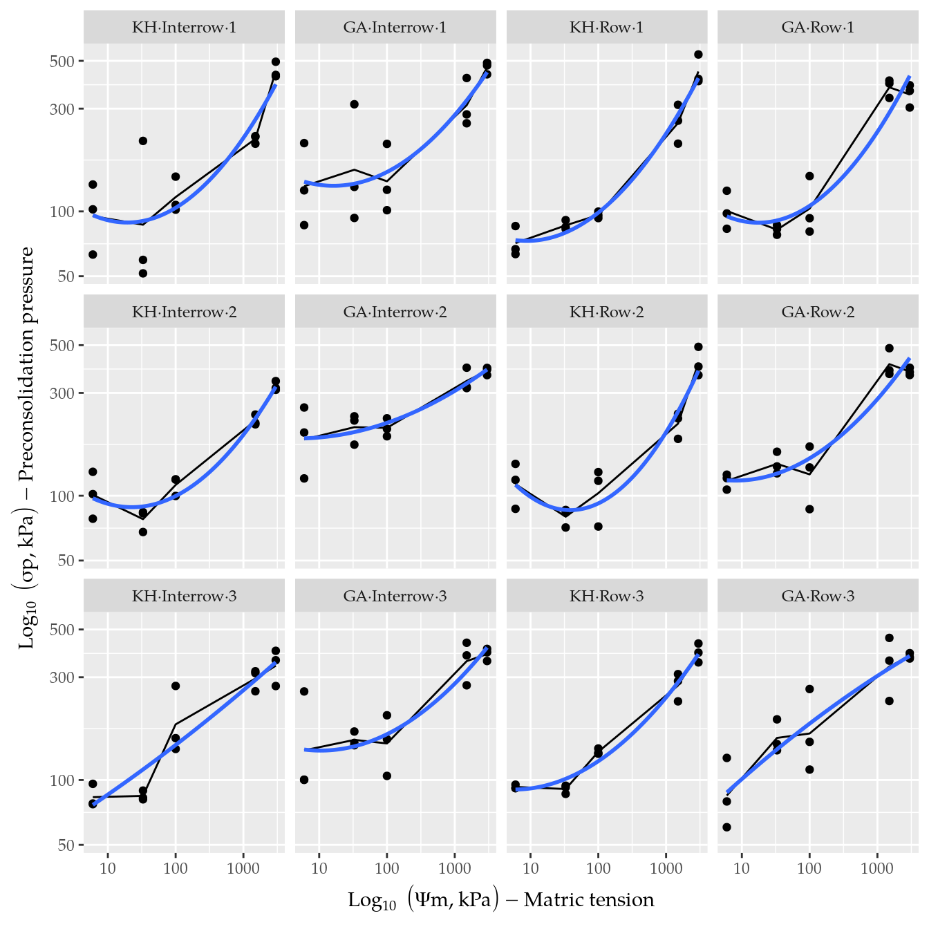
# Differnce in position mean profile conditional to other factors.
ggplot(data = da,
       mapping = aes(x = tensao, y = ppc, color = posi)) +
    facet_grid(facets = prof ~ solo) +
    geom_point() +
    stat_summary(geom = "line", fun.y = "mean") +
    scale_x_log10() +
    scale_y_log10() +
    labs(x = axis_text$tensao,
         y = axis_text$pcc,
         color = axis_text$posi)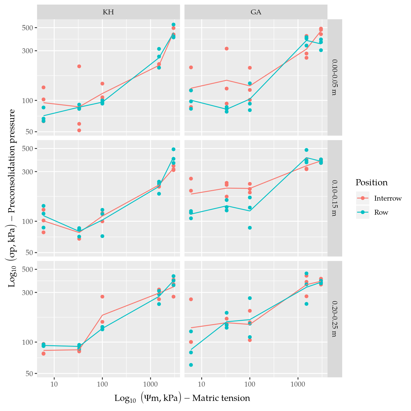
# Differnce in soil mean profile conditional to other factors.
ggplot(data = da,
       mapping = aes(x = tensao, y = ppc, color = solo)) +
    facet_grid(facets = prof ~ posi) +
    geom_point() +
    stat_summary(geom = "line", fun.y = "mean") +
    scale_x_log10() +
    scale_y_log10() +
    labs(x = axis_text$tensao,
         y = axis_text$pcc,
         color = axis_text$solo)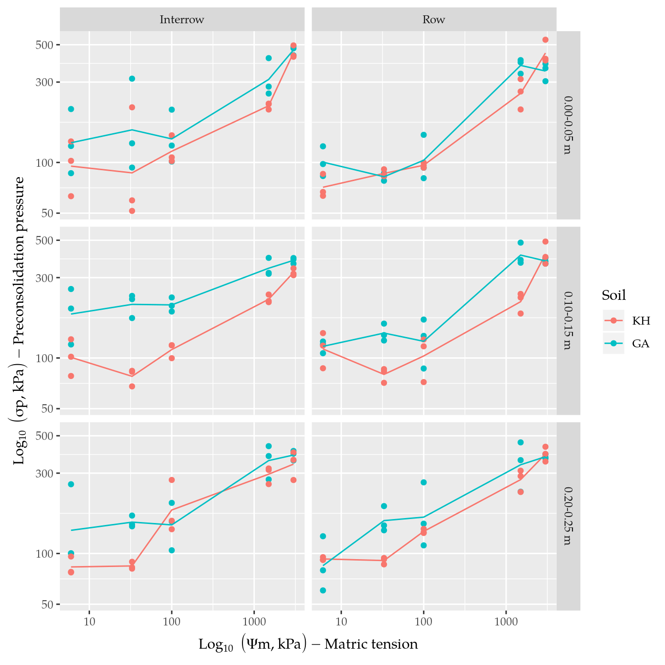
Linear mixed model
Based on exploratory data analysis, the effect of log of matric tension on log of preconsolidation pressure (response variable) can be properly described by a second order polynomial. Log of preconsolidation pressure was modelled as a function of soil type, sampling position, soil depth and log of matric tension. All interactions (until the 4th degree) were declared. The effect of experimental unit was accounted by random effets terms in intercept, slope and curvature of the linear mixed effects model. Likelihood ratio tests were performed to check the relevance random effects terms and Wald F tests were performed check the relevance of fixed effect terms, so those not relevant were abandoned getting a simpler model.
# Random intercept.
m0 <- lmer(logppc ~ solo * posi * prof * (logtensao + I(logtensao^2)) +
               (1 | ue), data = da)

# Variance of the random effects.
VarCorr(m0)
## Groups Name Std.Dev.
## ue (Intercept) 0.042762
## Residual 0.104107# Random intercept and slope.
m1 <- lmer(logppc ~ solo * posi * prof * (logtensao + I(logtensao^2)) +
(1 + logtensao | ue), data = da)## boundary (singular) fit: see ?isSingular# Variance of the random effects.
VarCorr(m1)## Groups Name Std.Dev. Corr
## ue (Intercept) 0.095690
## logtensao 0.021967 -1.000
## Residual 0.100321# Random intercept, slope and curvature.
m2 <- lmer(logppc ~ solo * posi * prof * (logtensao + I(logtensao^2)) +
(1 + logtensao + I(logtensao^2) | ue), data = da)
# Variance of the random effects.
VarCorr(m2)## Groups Name Std.Dev. Corr
## ue (Intercept) 0.083113
## logtensao 0.068131 -0.456
## I(logtensao^2) 0.017212 0.186 -0.959
## Residual 0.099456# Test of the extra parameters: variance of slope and/or curvature.
anova(m0, m1, m2)## refitting model(s) with ML (instead of REML)## Data: da
## Models:
## m0: logppc ~ solo * posi * prof * (logtensao + I(logtensao^2)) +
## m0: (1 | ue)
## m1: logppc ~ solo * posi * prof * (logtensao + I(logtensao^2)) +
## m1: (1 + logtensao | ue)
## m2: logppc ~ solo * posi * prof * (logtensao + I(logtensao^2)) +
## m2: (1 + logtensao + I(logtensao^2) | ue)
## Df AIC BIC logLik deviance Chisq Chi Df Pr(>Chisq)
## m0 38 -246.45 -125.12 161.23 -322.45
## m1 40 -246.75 -119.03 163.38 -326.75 4.2964 2 0.1167
## m2 43 -241.11 -103.81 163.55 -327.11 0.3580 3 0.9488anova(m0, m2)## refitting model(s) with ML (instead of REML)## Data: da
## Models:
## m0: logppc ~ solo * posi * prof * (logtensao + I(logtensao^2)) +
## m0: (1 | ue)
## m2: logppc ~ solo * posi * prof * (logtensao + I(logtensao^2)) +
## m2: (1 + logtensao + I(logtensao^2) | ue)
## Df AIC BIC logLik deviance Chisq Chi Df Pr(>Chisq)
## m0 38 -246.45 -125.12 161.23 -322.45
## m2 43 -241.11 -103.81 163.55 -327.11 4.6544 5 0.4595# Test for the fixed effect terms of the model.
anova(m0)## Type III Analysis of Variance Table with Satterthwaite's method
## Sum Sq Mean Sq NumDF DenDF F value
## solo 0.00471 0.00471 1 132.22 0.4345
## posi 0.00841 0.00841 1 132.22 0.7756
## prof 0.10354 0.05177 2 132.22 4.7768
## logtensao 0.14217 0.14217 1 120.00 13.1175
## I(logtensao^2) 0.77136 0.77136 1 120.00 71.1702
## solo:posi 0.04157 0.04157 1 132.22 3.8355
## solo:prof 0.01145 0.00573 2 132.22 0.5283
## posi:prof 0.00905 0.00453 2 132.22 0.4175
## solo:logtensao 0.01946 0.01946 1 120.00 1.7958
## solo:I(logtensao^2) 0.03373 0.03373 1 120.00 3.1123
## posi:logtensao 0.00083 0.00083 1 120.00 0.0768
## posi:I(logtensao^2) 0.00607 0.00607 1 120.00 0.5602
## prof:logtensao 0.12341 0.06170 2 120.00 5.6931
## prof:I(logtensao^2) 0.12517 0.06258 2 120.00 5.7743
## solo:posi:prof 0.04334 0.02167 2 132.22 1.9992
## solo:posi:logtensao 0.01736 0.01736 1 120.00 1.6016
## solo:posi:I(logtensao^2) 0.01139 0.01139 1 120.00 1.0510
## solo:prof:logtensao 0.03073 0.01537 2 120.00 1.4178
## solo:prof:I(logtensao^2) 0.03214 0.01607 2 120.00 1.4829
## posi:prof:logtensao 0.01316 0.00658 2 120.00 0.6071
## posi:prof:I(logtensao^2) 0.01654 0.00827 2 120.00 0.7630
## solo:posi:prof:logtensao 0.05301 0.02651 2 120.00 2.4455
## solo:posi:prof:I(logtensao^2) 0.05128 0.02564 2 120.00 2.3658
## Pr(>F)
## solo 0.5109119
## posi 0.3800758
## prof 0.0099309 **
## logtensao 0.0004299 ***
## I(logtensao^2) 8.627e-14 ***
## solo:posi 0.0522825 .
## solo:prof 0.5908258
## posi:prof 0.6595404
## solo:logtensao 0.1827520
## solo:I(logtensao^2) 0.0802474 .
## posi:logtensao 0.7821860
## posi:I(logtensao^2) 0.4556473
## prof:logtensao 0.0043439 **
## prof:I(logtensao^2) 0.0040335 **
## solo:posi:prof 0.1395142
## solo:posi:logtensao 0.2081329
## solo:posi:I(logtensao^2) 0.3073320
## solo:prof:logtensao 0.2462733
## solo:prof:I(logtensao^2) 0.2310985
## posi:prof:logtensao 0.5466042
## posi:prof:I(logtensao^2) 0.4685296
## solo:posi:prof:logtensao 0.0909917 .
## solo:posi:prof:I(logtensao^2) 0.0982379 .
## ---
## Signif. codes: 0 '***' 0.001 '**' 0.01 '*' 0.05 '.' 0.1 ' ' 1# No significant 4 degree interaction.
# No significant 3 degree interaction.
# No significant 2 degree with soil.
# No significant 2 degree with posi.
# Fitting a smaller model with relevant terms.
m3 <- update(m0, . ~ (solo + posi + prof) *
(logtensao + I(logtensao^2)) +
solo:posi +
(1 | ue))
anova(m0, m3)## refitting model(s) with ML (instead of REML)## Data: da
## Models:
## m3: logppc ~ solo + posi + prof + logtensao + I(logtensao^2) + (1 |
## m3: ue) + solo:logtensao + solo:I(logtensao^2) + posi:logtensao +
## m3: posi:I(logtensao^2) + prof:logtensao + prof:I(logtensao^2) +
## m3: solo:posi
## m0: logppc ~ solo * posi * prof * (logtensao + I(logtensao^2)) +
## m0: (1 | ue)
## Df AIC BIC logLik deviance Chisq Chi Df Pr(>Chisq)
## m3 18 -261.63 -204.16 148.81 -297.63
## m0 38 -246.45 -125.12 161.23 -322.45 24.825 20 0.2082anova(m3)## Type III Analysis of Variance Table with Satterthwaite's method
## Sum Sq Mean Sq NumDF DenDF F value Pr(>F)
## solo 0.00471 0.00471 1 147.82 0.4319 0.5120850
## posi 0.00841 0.00841 1 147.82 0.7709 0.3813661
## prof 0.10359 0.05179 2 147.82 4.7475 0.0100387
## logtensao 0.14217 0.14217 1 134.00 13.0316 0.0004316
## I(logtensao^2) 0.77136 0.77136 1 134.00 70.7041 5.409e-14
## solo:logtensao 0.01946 0.01946 1 134.00 1.7840 0.1839177
## solo:I(logtensao^2) 0.03373 0.03373 1 134.00 3.0919 0.0809649
## posi:logtensao 0.00083 0.00083 1 134.00 0.0763 0.7828322
## posi:I(logtensao^2) 0.00607 0.00607 1 134.00 0.5565 0.4569709
## prof:logtensao 0.12341 0.06170 2 134.00 5.6558 0.0043842
## prof:I(logtensao^2) 0.12517 0.06258 2 134.00 5.7365 0.0040700
## solo:posi 0.04024 0.04024 1 30.00 3.6888 0.0643284
##
## solo
## posi
## prof *
## logtensao ***
## I(logtensao^2) ***
## solo:logtensao
## solo:I(logtensao^2) .
## posi:logtensao
## posi:I(logtensao^2)
## prof:logtensao **
## prof:I(logtensao^2) **
## solo:posi .
## ---
## Signif. codes: 0 '***' 0.001 '**' 0.01 '*' 0.05 '.' 0.1 ' ' 1The model with random effets in the intercept were not inferior, by the likelihood ratio test, to those more complex that included random effects for slope and curvature. So, the selected model has random effects of experimental units on the intercept only.
From this model, by Wald F tests, there weren’t 4th degree signficant interactions neither 3rd degree. There were 2nd degree signficant interactions involving soil or position at 10%, and involving depth at less than 1%. All two way interactions were kept except those involving depth and soil or depth and position. So, depth and soil have additive effect, the same for depth and position.
Curve comparison
# Estimated marginal means with covariate set at 1.
emm <- emmeans(m3,
               specs = ~solo + posi + prof,
               at = list(logtensao = 1))

# Get experimental points and matrix to calculate marginal means.
grid <- attr(emm, "grid")
L <- attr(emm, "linfct")

# Fixed effects estimates.
b <- fixef(m3)

# Zero order terms (intercept).
ord0 <- names(b) %>%
    # grep(pattern = "logtensao", value = TRUE, invert = TRUE)
    grepl(pattern = "logtensao") %>% `!`()

# First order terms (slope).
ord1 <- names(b) %>%
    # grep(pattern = "logtensao$", value = TRUE, invert = FALSE)
    grepl(pattern = "logtensao$")

# Second order terms (curvatures).
ord2 <- names(b) %>%
    # grep(pattern = "I\\(logtensao\\^2\\)$", value = TRUE, invert = FALSE)
    grepl(pattern = "I\\(logtensao\\^2\\)$")

# Get the equation coefficients: b0 + b1 * x + b2 * x^2.
grid$b0 <- c(L %*% (b * ord0))
grid$b1 <- c(L %*% (b * ord1))
grid$b2 <- c(L %*% (b * ord2))

grid <- grid %>%
    mutate(label = sprintf("'%0.2f' %s '%0.3f' * x %s '%0.4f' * x^2",
                           b0,
                           ifelse(b1 >= 0, "+", "-"),
                           abs(b1),
                           ifelse(b2 >= 0, "+", "-"),
                           abs(b2)))


# Table of equation coefficients for each experimental point.
grid
## solo posi prof .wgt. b0 b1 b2
## 1 KH Interrow 0.00-0.05 m 15 2.130988 -0.338850092 0.13352557
## 2 GA Interrow 0.00-0.05 m 15 2.230424 -0.212148979 0.09589438
## 3 KH Row 0.00-0.05 m 15 2.092622 -0.365048580 0.14949081
## 4 GA Row 0.00-0.05 m 15 2.111166 -0.238347467 0.11185963
## 5 KH Interrow 0.10-0.15 m 15 2.235905 -0.329616267 0.11862226
## 6 GA Interrow 0.10-0.15 m 15 2.335341 -0.202915154 0.08099108
## 7 KH Row 0.10-0.15 m 15 2.197539 -0.355814755 0.13458751
## 8 GA Row 0.10-0.15 m 15 2.216083 -0.229113642 0.09695632
## 9 KH Interrow 0.20-0.25 m 15 1.904498 0.004061914 0.05027863
## 10 GA Interrow 0.20-0.25 m 15 2.003934 0.130763027 0.01264745
## 11 KH Row 0.20-0.25 m 15 1.866132 -0.022136574 0.06624388
## 12 GA Row 0.20-0.25 m 15 1.884676 0.104564539 0.02861270
## label
## 1 '2.13' - '0.339' * x + '0.1335' * x^2
## 2 '2.23' - '0.212' * x + '0.0959' * x^2
## 3 '2.09' - '0.365' * x + '0.1495' * x^2
## 4 '2.11' - '0.238' * x + '0.1119' * x^2
## 5 '2.24' - '0.330' * x + '0.1186' * x^2
## 6 '2.34' - '0.203' * x + '0.0810' * x^2
## 7 '2.20' - '0.356' * x + '0.1346' * x^2
## 8 '2.22' - '0.229' * x + '0.0970' * x^2
## 9 '1.90' + '0.004' * x + '0.0503' * x^2
## 10 '2.00' + '0.131' * x + '0.0126' * x^2
## 11 '1.87' - '0.022' * x + '0.0662' * x^2
## 12 '1.88' + '0.105' * x + '0.0286' * x^2The above table has the estimated curve coefficients for each experimental point resulted of combining soil, position and depth levels. The fitted curve has equation \[ y = \beta_0 + \beta_1 x + \beta_2 x^2 \] where \(y\) is the (conditional mean of) log 10 of preconsolidation pressure, \(x\) is the log 10 of matric tension and \(\beta_0\), \(\beta_1\) and \(\beta_2\) are intercept, slope and curvature parameter of the second order polynomial.
# To compare curves with Wald F test statistic.
compare_curves <- function(index, levels = NULL) {
    J <- L[index, , drop = FALSE]
    K <- wzRfun::apc(J, lev = levels)
    f_test <- apply(K[, , drop = FALSE],
                    MARGIN = 1,
                    FUN = function(Ki) {
                        U <- rbind(Ki %*% diag(ord0),
                                   Ki %*% diag(ord1),
                                   Ki %*% diag(ord2))
                        f_test <-
                            linearHypothesis(model = m3,
                                             hypothesis.matrix = U,
                                             test = "F")
                        tail(f_test[, c("F", "Pr(>F)")], n = 1)
                    })
    f_test <- do.call(what = rbind, args = f_test)
    cbind(contrast = rownames(f_test), f_test)
}

# Tests of soil curves are equal in each posi:prof combination.
grid %>%
    mutate(row = 1:n()) %>%
    group_by(posi, prof) %>%
    do({
        compare_curves(.$row, .$solo)
    }) %>%
    as.data.frame()
## posi prof contrast F Pr(>F)
## 1 Interrow 0.00-0.05 m KH-GA 12.291555 7.688935e-07
## 2 Interrow 0.10-0.15 m KH-GA 12.291555 7.688935e-07
## 3 Interrow 0.20-0.25 m KH-GA 12.291555 7.688935e-07
## 4 Row 0.00-0.05 m KH-GA 5.222928 2.240331e-03
## 5 Row 0.10-0.15 m KH-GA 5.222928 2.240331e-03
## 6 Row 0.20-0.25 m KH-GA 5.222928 2.240331e-03# Tests of posi curves are equal in each soil:prof combination.
grid %>%
mutate(row = 1:n()) %>%
group_by(solo, prof) %>%
do({
compare_curves(.$row, .$posi)
}) %>%
as.data.frame()## solo prof contrast F Pr(>F)
## 1 KH 0.00-0.05 m Interrow-Row 2.831772 0.042593695
## 2 KH 0.10-0.15 m Interrow-Row 2.831772 0.042593695
## 3 KH 0.20-0.25 m Interrow-Row 2.831772 0.042593695
## 4 GA 0.00-0.05 m Interrow-Row 5.436113 0.001731259
## 5 GA 0.10-0.15 m Interrow-Row 5.436113 0.001731259
## 6 GA 0.20-0.25 m Interrow-Row 5.436113 0.001731259# grid %>%
# mutate(row = 1:n()) %>%
# group_by(solo, posi) %>%
# do({
# compare_curves(.$row, as.integer(.$prof))
# }) %>%
# as.data.frame()Wald F test were applied to test with two curves are equal. The null hypothesis states that all three parameters (\(\beta_0\), \(\beta_1\), \(\beta_2\)) are simultaneous equal for a pair of curves \[ H_0: \begin{bmatrix} \beta_0 \\ \beta_1 \\ \beta_2 \end{bmatrix} = \begin{bmatrix} \beta_0' \\ \beta_1' \\ \beta_2' \end{bmatrix}. \]
The tables above shows the F statistics and associate p-value to test the equality of two curves using the Wald test. Curves from soils were compared for each position and depth combination (6 conditions). Because there wasn’t 3rd order interaction, the F statistic is the same for all depth at the same position. The greater difference, as showed by the curves on the next graphics, is between soil curves at interrow position.
The same test were applied to test equality of curves between position for each soil and depth combination (6 conditions). Because there wasn’t 3rd order interaction, the F statistic is the same for all depth at the same soil. The greater difference, as showed by the curves on the next graphics, is between position curves at GA soil. Despite the overlapping of confidence bands between position in the KH soil, according two the F test, these curves are not equal at 5%.
# Conditions to get estimated values.
pred <- with(da,
             expand.grid(solo = levels(solo),
                         posi = levels(posi),
                         prof = levels(prof),
                         logtensao = seq(0.5, 3.5, length = 31),
                         KEEP.OUT.ATTRS = FALSE))

# Model matrix for prediction.
X <- model.matrix(formula(terms(m3))[-2], data = pred)

# Checks.
stopifnot(ncol(X) == length(fixef(m3)))
stopifnot(all(colnames(X) == names(fixef(m3))))

# Predicted value.
pred$fit <- X %*% fixef(m3)

# Standard error of predicted values.
pred$se <- sqrt(diag(X %*% tcrossprod(vcov(m3), X)))

# Quantile of t distribution.
qtl <- qt(p = 0.975, df = df.residual(m3))

# Confidence limits for predicted value.
pred$lwr <- pred$fit - qtl * pred$se
pred$upr <- pred$fit + qtl * pred$se

# Adds the equation to annotate on graphics.
grid <- grid %>%
    mutate(xpos = 2.5,
           ypos = ifelse(solo == "GA", 500, 400) - 30,
           hjust = c(0),
           vjust = c(0))

# Fitted curves with confidence bands and observed data.
# Soil in evidence.
ggplot(data = da,
       mapping = aes(x = tensao, y = ppc, color = solo)) +
    facet_grid(facets = prof ~ posi) +
    geom_point() +
    scale_x_log10() +
    scale_y_log10() +
    geom_line(data = pred,
              mapping = aes(x = 10^logtensao,
                            y = 10^fit,
                            color = solo)) +
    geom_smooth(data = pred,
                mapping = aes(x = 10^logtensao,
                              y = 10^fit,
                              ymin = 10^lwr,
                              ymax = 10^upr),
                stat = "identity",
                show.legend = FALSE) +
    geom_text(data = grid,
              mapping = aes(x = xpos,
                            y = ypos,
                            label = label,
                            hjust = hjust,
                            vjust = vjust),
              show.legend = FALSE,
              parse = TRUE) +
    labs(x = axis_text$tensao,
         y = axis_text$pcc,
         color = axis_text$solo)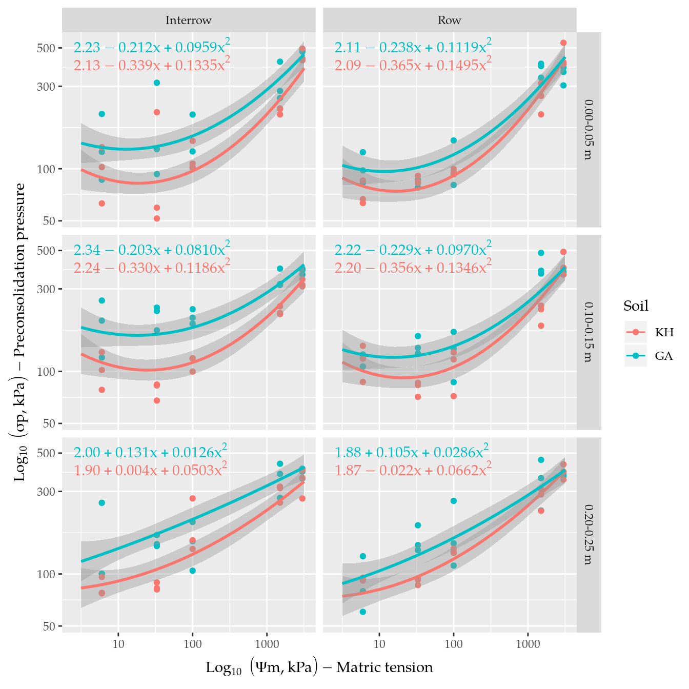
grid <- grid %>%
    mutate(xpos = 2.5,
           ypos = ifelse(posi == "Interrow", 500, 400) - 30)

# Fitted curves with confidence bands and observed data.
# Position in evidence.
ggplot(data = da,
       mapping = aes(x = tensao, y = ppc, color = posi)) +
    facet_grid(facets = prof ~ solo) +
    geom_point() +
    scale_x_log10() +
    scale_y_log10() +
    geom_line(data = pred,
              mapping = aes(x = 10^logtensao,
                            y = 10^fit,
                            color = posi)) +
    geom_smooth(data = pred,
                mapping = aes(x = 10^logtensao,
                              y = 10^fit,
                              ymin = 10^lwr,
                              ymax = 10^upr),
                stat = "identity",
                show.legend = FALSE) +
    geom_text(data = grid,
              mapping = aes(x = xpos,
                            y = ypos,
                            label = label,
                            hjust = hjust,
                            vjust = vjust),
              show.legend = FALSE,
              parse = TRUE) +
    labs(x = axis_text$tensao,
         y = axis_text$pcc,
         color = axis_text$posi)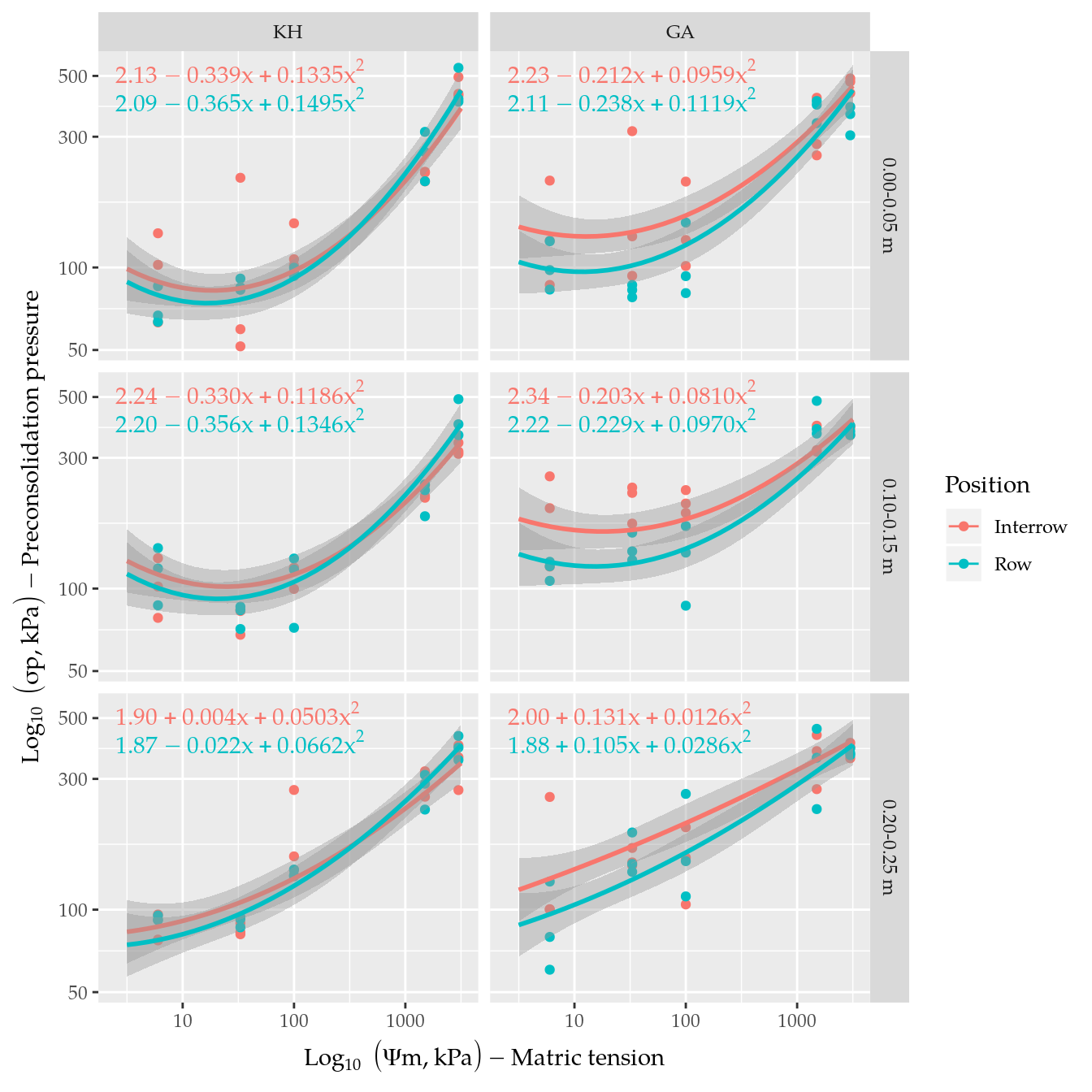
The above graphics displays the estimated quadratic curve fitted (solid line) in each combination of soil, position and depth to describe log of preconsolidation pressure as a function of log matric tension. The shaded region wrapping the estimated curve is the confidence band for the fitted conditional mean. The equations inside each cell plot are in log-log scale. By visualizing the curves, we notice that the predicted value for each soil differ at most part of the matric tension domain. The difference is greater in the interrow position than in row, as stated by the R test previous applied. The difference is the same in all depth at the same position level, since there wasn’t 3rd degree interaction involving soil, position and depth.
Session information
## Atualizado em 19 de julho de 2019.
##
## R version 3.6.1 (2019-07-05)
## Platform: x86_64-pc-linux-gnu (64-bit)
## Running under: Ubuntu 18.04.2 LTS
##
## Matrix products: default
## BLAS:   /usr/lib/x86_64-linux-gnu/blas/libblas.so.3.7.1
## LAPACK: /usr/lib/x86_64-linux-gnu/lapack/liblapack.so.3.7.1
##
## locale:
##  [1] LC_CTYPE=pt_BR.UTF-8       LC_NUMERIC=C
##  [3] LC_TIME=pt_BR.UTF-8        LC_COLLATE=en_US.UTF-8
##  [5] LC_MONETARY=pt_BR.UTF-8    LC_MESSAGES=en_US.UTF-8
##  [7] LC_PAPER=pt_BR.UTF-8       LC_NAME=C
##  [9] LC_ADDRESS=C               LC_TELEPHONE=C
## [11] LC_MEASUREMENT=pt_BR.UTF-8 LC_IDENTIFICATION=C
##
## attached base packages:
## [1] stats     graphics  grDevices utils     datasets  methods
## [7] base
##
## other attached packages:
##  [1] forcats_0.4.0       stringr_1.4.0       dplyr_0.8.3
##  [4] purrr_0.3.2         readr_1.3.1         tidyr_0.8.3
##  [7] tibble_2.1.3        ggplot2_3.2.0       tidyverse_1.2.1
## [10] car_3.0-3           carData_3.0-2       emmeans_1.3.5.1
## [13] lmerTest_3.1-0      lme4_1.1-21         Matrix_1.2-17
## [16] EACS_0.0-8          wzRfun_0.91         captioner_2.2.3
## [19] latticeExtra_0.6-28 RColorBrewer_1.1-2  lattice_0.20-38
## [22] knitr_1.23
##
## loaded via a namespace (and not attached):
##  [1] TH.data_1.0-10      minqa_1.2.4         colorspace_1.4-1
##  [4] rio_0.5.16          rprojroot_1.3-2     estimability_1.3
##  [7] fs_1.3.1            rstudioapi_0.10     roxygen2_6.1.1
## [10] remotes_2.1.0       mvtnorm_1.0-11      lubridate_1.7.4
## [13] xml2_1.2.0          codetools_0.2-16    splines_3.6.1
## [16] pkgload_1.0.2       zeallot_0.1.0       jsonlite_1.6
## [19] nloptr_1.2.1        pbkrtest_0.4-7      broom_0.5.2
## [22] compiler_3.6.1      httr_1.4.0          backports_1.1.4
## [25] assertthat_0.2.1    lazyeval_0.2.2      cli_1.1.0
## [28] htmltools_0.3.6     prettyunits_1.0.2   tools_3.6.1
## [31] coda_0.19-3         gtable_0.3.0        glue_1.3.1
## [34] reshape2_1.4.3      Rcpp_1.0.1          cellranger_1.1.0
## [37] pkgdown_1.3.0       vctrs_0.2.0         nlme_3.1-140
## [40] xfun_0.8            ps_1.3.0            openxlsx_4.1.0.1
## [43] testthat_2.1.1      rvest_0.3.4         devtools_2.1.0
## [46] MASS_7.3-51.4       zoo_1.8-6           scales_1.0.0
## [49] hms_0.5.0           parallel_3.6.1      sandwich_2.5-1
## [52] yaml_2.2.0          curl_3.3            memoise_1.1.0
## [55] stringi_1.4.3       desc_1.2.0          boot_1.3-23
## [58] pkgbuild_1.0.3      zip_2.0.3           rlang_0.4.0
## [61] pkgconfig_2.0.2     commonmark_1.7      evaluate_0.14
## [64] labeling_0.3        processx_3.4.0      tidyselect_0.2.5
## [67] plyr_1.8.4          magrittr_1.5        R6_2.4.0
## [70] generics_0.0.2      multcomp_1.4-10     pillar_1.4.2
## [73] haven_2.1.1         foreign_0.8-71      withr_2.1.2
## [76] survival_2.44-1.1   abind_1.4-5         modelr_0.1.4
## [79] crayon_1.3.4        rmarkdown_1.13      usethis_1.5.1
## [82] grid_3.6.1          readxl_1.3.1        data.table_1.12.2
## [85] callr_3.3.0         digest_0.6.20       xtable_1.8-4
## [88] numDeriv_2016.8-1.1 munsell_0.5.0       sessioninfo_1.1.1