Capítulo 14 Blocos incompletos tipo I e II

Figura 14.1: Ilustração de um experimento em delineamento de blocos incompletos balanceados tipo 1. Os 15 pensonagens de Os Simpsons são os blocos arranjados em 5 repetições. Em cada repetição cada tratamento aparece uma vez. Cada bloco contém 2 tratamentos. Este delineamento possui \(t = 6\) tratamentos, bloco de tamanho \(k = 2\), \(r = 5\) repetições, \(b = 15\) blocos, \(\lambda = 1\) ocorrência simultânea de cada par e eficiência de 0,6.

Figura 14.2: Ilustração de um experimento em delineamento de blocos incompletos balanceados tipo 2. Os 15 pensonagens de Os Simpsons são os blocos arranjados em 5 grupos de repetições. Em um grupo cada tratamento aparece duas vezes. Cada bloco contém 4 tratamentos. Este delineamento possui \(t = 6\) tratamentos, bloco de tamanho \(k = 4\), \(r = 10\) repetições, \(b = 15\) blocos, \(\lambda = 6\) ocorrências simultâneas de cada par e eficiência de 0,9.
ATTENTION: quando não se tem efeito de bloco dentro de repetições, poderia-se pensar em fazer um experimento em blocos completos. IMPROVE.
URL: http://leg.ufpr.br/~walmes/cursoR/cnpaf/cap09bib-iso.R
ATTENTION: o tipo I e II podem ser tipo III se ignorar a estrutura agrupara de blocos em repetições ou grupos de repetições.
library(car)       # Anova().
library(emmeans)   # emmeans().
library(multcomp)  # glht().
library(lme4)      # lmer().
library(lmerTest)  # anova() e summary() para classe lmerMod.
library(HH)        # mmc() e mmcplot().
library(tidyverse) # Manipulação e visualização.

# Funções.
source("mpaer_functions.R")
14.1 Bloco incompleto tipo I
O objeto PimentelTb10.3.1 contém dados de um experimento em blocos incompletos tipo I (PIMENTEL-GOMES (2009), p.185). Em cada repetição (rept), os tratamentos (trat) aparecem uma vez dispostos em 4 blocos (bloc) de tamanho 2. Ao todo, são 7 repetições de cada tratamento.
14.1.1 Modelo de efeitos fixos
# Experimento em BIB tipo I.
da <- as_tibble(labestData::PimentelTb10.3.1)
str(da)
## Classes 'tbl_df', 'tbl' and 'data.frame': 56 obs. of 4 variables:
## $ rept: Factor w/ 7 levels "1","2","3","4",..: 1 1 1 1 1 1 1 1 2 2 ...
## $ trat: Factor w/ 8 levels "1","2","3","4",..: 1 2 3 4 5 6 7 8 1 3 ...
## $ bloc: Factor w/ 4 levels "1","2","3","4": 1 1 2 2 3 3 4 4 1 1 ...
## $ y : int 20 18 15 16 14 15 16 18 24 18 ...# # Número de parcelas com cada tratamento.
# with(da, table(trat))
#
# # Número de blocos por repetição.
# with(da, table(rept, bloc))
#
# # Cada tratamento ocorre uma vez com outro.
# with(da, table(rept:bloc, trat))
# Repetições, blocos e tratamentos.
with(da, table(bloc, trat, rept)) %>%
addmargins(margin = 1:2) %>%
print.table(zero.print = ".")## , , rept = 1
##
## trat
## bloc 1 2 3 4 5 6 7 8 Sum
## 1 1 1 . . . . . . 2
## 2 . . 1 1 . . . . 2
## 3 . . . . 1 1 . . 2
## 4 . . . . . . 1 1 2
## Sum 1 1 1 1 1 1 1 1 8
##
## , , rept = 2
##
## trat
## bloc 1 2 3 4 5 6 7 8 Sum
## 1 1 . 1 . . . . . 2
## 2 . 1 . . . . . 1 2
## 3 . . . 1 1 . . . 2
## 4 . . . . . 1 1 . 2
## Sum 1 1 1 1 1 1 1 1 8
##
## , , rept = 3
##
## trat
## bloc 1 2 3 4 5 6 7 8 Sum
## 1 1 . . 1 . . . . 2
## 2 . 1 . . . . 1 . 2
## 3 . . 1 . . 1 . . 2
## 4 . . . . 1 . . 1 2
## Sum 1 1 1 1 1 1 1 1 8
##
## , , rept = 4
##
## trat
## bloc 1 2 3 4 5 6 7 8 Sum
## 1 1 . . . 1 . . . 2
## 2 . 1 1 . . . . . 2
## 3 . . . 1 . . 1 . 2
## 4 . . . . . 1 . 1 2
## Sum 1 1 1 1 1 1 1 1 8
##
## , , rept = 5
##
## trat
## bloc 1 2 3 4 5 6 7 8 Sum
## 1 1 . . . . 1 . . 2
## 2 . 1 . 1 . . . . 2
## 3 . . 1 . . . . 1 2
## 4 . . . . 1 . 1 . 2
## Sum 1 1 1 1 1 1 1 1 8
##
## , , rept = 6
##
## trat
## bloc 1 2 3 4 5 6 7 8 Sum
## 1 1 . . . . . 1 . 2
## 2 . 1 . . . 1 . . 2
## 3 . . 1 . 1 . . . 2
## 4 . . . 1 . . . 1 2
## Sum 1 1 1 1 1 1 1 1 8
##
## , , rept = 7
##
## trat
## bloc 1 2 3 4 5 6 7 8 Sum
## 1 1 . . . . . . 1 2
## 2 . 1 . . 1 . . . 2
## 3 . . 1 . . . 1 . 2
## 4 . . . 1 . 1 . . 2
## Sum 1 1 1 1 1 1 1 1 8O necessário para haver estimabilidade é conectividade.
library(igraph)

edg <- by(data = da$trat,
          INDICES = interaction(da$rept, da$bloc),
          FUN = combn,
          m = 2) %>%
    flatten_int()

ghp <- graph(edg, directed = FALSE)
plot(ghp,
     layout = layout_in_circle,
     edge.curved = FALSE)
# Análise gráfica.
ggplot(data = da,
mapping = aes(x = trat, y = y, color = bloc)) +
facet_wrap(facets = ~rept) +
geom_point()
A análise intrabloco considera que o efeito de bloco dentro de repetição é fixo.
Usando terms() declaramos a sequência das fontes de variação no quadro de anova.
# Ajuste do modelo.
m0 <- lm(terms(y ~ rept/bloc + trat, keep.order = TRUE),
         data = da)

# Checagem dos pressupostos.
par(mfrow = c(2, 2)); plot(m0); layout(1)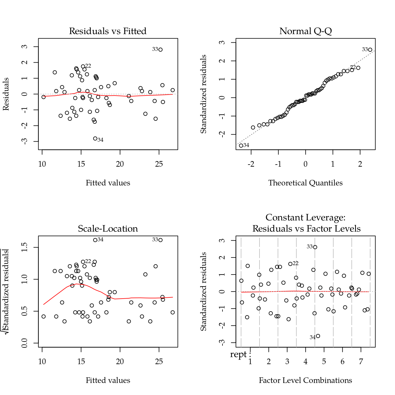
# Quadro de análise de variância (hipóteses sequenciais).
anova(m0)
## Analysis of Variance Table
##
## Response: y
## Df Sum Sq Mean Sq F value Pr(>F)
## rept 6 102.46 17.077 5.5067 0.001468 **
## rept:bloc 21 422.88 20.137 6.4933 3.458e-05 ***
## trat 7 376.37 53.768 17.3378 2.055e-07 ***
## Residuals 21 65.13 3.101
## ---
## Signif. codes: 0 '***' 0.001 '**' 0.01 '*' 0.05 '.' 0.1 ' ' 1# Quadro de análise de variância (hipóteses marginais).
Anova(m0)## Anova Table (Type II tests)
##
## Response: y
## Sum Sq Df F value Pr(>F)
## rept 102.46 6 5.5067 0.001468 **
## rept:bloc 96.41 21 1.4804 0.187952
## trat 376.37 7 17.3378 2.055e-07 ***
## Residuals 65.13 21
## ---
## Signif. codes: 0 '***' 0.001 '**' 0.01 '*' 0.05 '.' 0.1 ' ' 1# Resultado idem ao anterior (o procedimento interno não é).
drop1(m0, scope = . ~ ., test = "F")## Single term deletions
##
## Model:
## y ~ rept/bloc + trat
## Df Sum of Sq RSS AIC F value Pr(>F)
## <none> 65.13 78.454
## rept 6 45.21 110.33 95.977 2.4296 0.06089 .
## trat 7 376.37 441.50 171.630 17.3378 2.055e-07 ***
## rept:bloc 21 96.41 161.54 87.325 1.4804 0.18795
## ---
## Signif. codes: 0 '***' 0.001 '**' 0.01 '*' 0.05 '.' 0.1 ' ' 1# Médias marginais ajustadas.
emm <- emmeans(m0, specs = ~trat)## NOTE: A nesting structure was detected in the fitted model:
## bloc %in% reptemm## trat emmean SE df lower.CL upper.CL
## 1 23.3 0.857 21 21.5 25.1
## 2 22.7 0.857 21 20.9 24.5
## 3 16.4 0.857 21 14.7 18.2
## 4 14.2 0.857 21 12.4 16.0
## 5 14.4 0.857 21 12.7 16.2
## 6 14.9 0.857 21 13.2 16.7
## 7 15.8 0.857 21 14.0 17.6
## 8 15.7 0.857 21 13.9 17.5
##
## Results are averaged over the levels of: bloc, rept
## Confidence level used: 0.95grid <- attr(emm, "grid")
L <- attr(emm, "linfct")
rownames(L) <- grid[[1]]
MASS::fractions(t(L))## 1 2 3 4 5 6 7 8
## (Intercept) 1 1 1 1 1 1 1 1
## rept2 1/7 1/7 1/7 1/7 1/7 1/7 1/7 1/7
## rept3 1/7 1/7 1/7 1/7 1/7 1/7 1/7 1/7
## rept4 1/7 1/7 1/7 1/7 1/7 1/7 1/7 1/7
## rept5 1/7 1/7 1/7 1/7 1/7 1/7 1/7 1/7
## rept6 1/7 1/7 1/7 1/7 1/7 1/7 1/7 1/7
## rept7 1/7 1/7 1/7 1/7 1/7 1/7 1/7 1/7
## rept1:bloc2 1/28 1/28 1/28 1/28 1/28 1/28 1/28 1/28
## rept2:bloc2 1/28 1/28 1/28 1/28 1/28 1/28 1/28 1/28
## rept3:bloc2 1/28 1/28 1/28 1/28 1/28 1/28 1/28 1/28
## rept4:bloc2 1/28 1/28 1/28 1/28 1/28 1/28 1/28 1/28
## rept5:bloc2 1/28 1/28 1/28 1/28 1/28 1/28 1/28 1/28
## rept6:bloc2 1/28 1/28 1/28 1/28 1/28 1/28 1/28 1/28
## rept7:bloc2 1/28 1/28 1/28 1/28 1/28 1/28 1/28 1/28
## rept1:bloc3 1/28 1/28 1/28 1/28 1/28 1/28 1/28 1/28
## rept2:bloc3 1/28 1/28 1/28 1/28 1/28 1/28 1/28 1/28
## rept3:bloc3 1/28 1/28 1/28 1/28 1/28 1/28 1/28 1/28
## rept4:bloc3 1/28 1/28 1/28 1/28 1/28 1/28 1/28 1/28
## rept5:bloc3 1/28 1/28 1/28 1/28 1/28 1/28 1/28 1/28
## rept6:bloc3 1/28 1/28 1/28 1/28 1/28 1/28 1/28 1/28
## rept7:bloc3 1/28 1/28 1/28 1/28 1/28 1/28 1/28 1/28
## rept1:bloc4 1/28 1/28 1/28 1/28 1/28 1/28 1/28 1/28
## rept2:bloc4 1/28 1/28 1/28 1/28 1/28 1/28 1/28 1/28
## rept3:bloc4 1/28 1/28 1/28 1/28 1/28 1/28 1/28 1/28
## rept4:bloc4 1/28 1/28 1/28 1/28 1/28 1/28 1/28 1/28
## rept5:bloc4 1/28 1/28 1/28 1/28 1/28 1/28 1/28 1/28
## rept6:bloc4 1/28 1/28 1/28 1/28 1/28 1/28 1/28 1/28
## rept7:bloc4 1/28 1/28 1/28 1/28 1/28 1/28 1/28 1/28
## trat2 0 1 0 0 0 0 0 0
## trat3 0 0 1 0 0 0 0 0
## trat4 0 0 0 1 0 0 0 0
## trat5 0 0 0 0 1 0 0 0
## trat6 0 0 0 0 0 1 0 0
## trat7 0 0 0 0 0 0 1 0
## trat8 0 0 0 0 0 0 0 1# Contrastes de tukey.
glht0 <- summary(glht(m0, linfct = mcp(trat = "Tukey")),
test = adjusted(type = "fdr"))
glht0##
## Simultaneous Tests for General Linear Hypotheses
##
## Multiple Comparisons of Means: Tukey Contrasts
##
##
## Fit: lm(formula = terms(y ~ rept/bloc + trat, keep.order = TRUE),
## data = da)
##
## Linear Hypotheses:
## Estimate Std. Error t value Pr(>|t|)
## 2 - 1 == 0 -0.625 1.245 -0.502 0.695463
## 3 - 1 == 0 -6.875 1.245 -5.521 4.51e-05 ***
## 4 - 1 == 0 -9.125 1.245 -7.328 6.98e-06 ***
## 5 - 1 == 0 -8.875 1.245 -7.127 6.98e-06 ***
## 6 - 1 == 0 -8.375 1.245 -6.726 8.23e-06 ***
## 7 - 1 == 0 -7.500 1.245 -6.023 1.96e-05 ***
## 8 - 1 == 0 -7.625 1.245 -6.123 1.79e-05 ***
## 3 - 2 == 0 -6.250 1.245 -5.019 0.000134 ***
## 4 - 2 == 0 -8.500 1.245 -6.826 8.23e-06 ***
## 5 - 2 == 0 -8.250 1.245 -6.625 8.23e-06 ***
## 6 - 2 == 0 -7.750 1.245 -6.224 1.67e-05 ***
## 7 - 2 == 0 -6.875 1.245 -5.521 4.51e-05 ***
## 8 - 2 == 0 -7.000 1.245 -5.621 4.37e-05 ***
## 4 - 3 == 0 -2.250 1.245 -1.807 0.183355
## 5 - 3 == 0 -2.000 1.245 -1.606 0.246357
## 6 - 3 == 0 -1.500 1.245 -1.205 0.398192
## 7 - 3 == 0 -0.625 1.245 -0.502 0.695463
## 8 - 3 == 0 -0.750 1.245 -0.602 0.673733
## 5 - 4 == 0 0.250 1.245 0.201 0.874028
## 6 - 4 == 0 0.750 1.245 0.602 0.673733
## 7 - 4 == 0 1.625 1.245 1.305 0.384568
## 8 - 4 == 0 1.500 1.245 1.205 0.398192
## 6 - 5 == 0 0.500 1.245 0.402 0.745322
## 7 - 5 == 0 1.375 1.245 1.104 0.438655
## 8 - 5 == 0 1.250 1.245 1.004 0.481729
## 7 - 6 == 0 0.875 1.245 0.703 0.673733
## 8 - 6 == 0 0.750 1.245 0.602 0.673733
## 8 - 7 == 0 -0.125 1.245 -0.100 0.920992
## ---
## Signif. codes: 0 '***' 0.001 '**' 0.01 '*' 0.05 '.' 0.1 ' ' 1
## (Adjusted p values reported -- fdr method)# Exibição compacta com letras.
cld(glht0)## 1 2 3 4 5 6 7 8
## "b" "b" "a" "a" "a" "a" "a" "a"# Gráfico dos intervalos para os contrastes.
plot(glht0)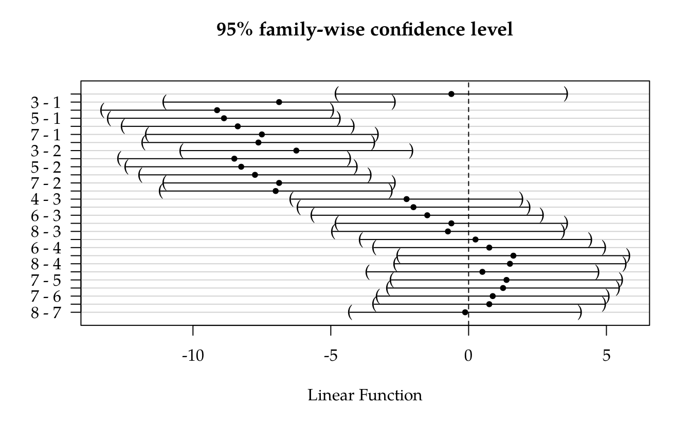
# Resultados para colocar em gráfico de segmentos.
results_m0 <- wzRfun::apmc(L,
                           model = m0,
                           focus = "trat",
                           test = "fdr")

# Gráfico de segmentos para as estimativas intervalares.
ggplot(data = results_m0,
       mapping = aes(x = fit, y = reorder(trat, fit))) +
    geom_point() +
    geom_errorbarh(mapping = aes(xmin = lwr, xmax = upr),
                   height = 0) +
    geom_text(mapping = aes(label = sprintf("%0.1f%s", fit, cld)),
              vjust = 0,
              nudge_y = 0.07) +
    labs(x = "Produção",
         y = "Tratamentos")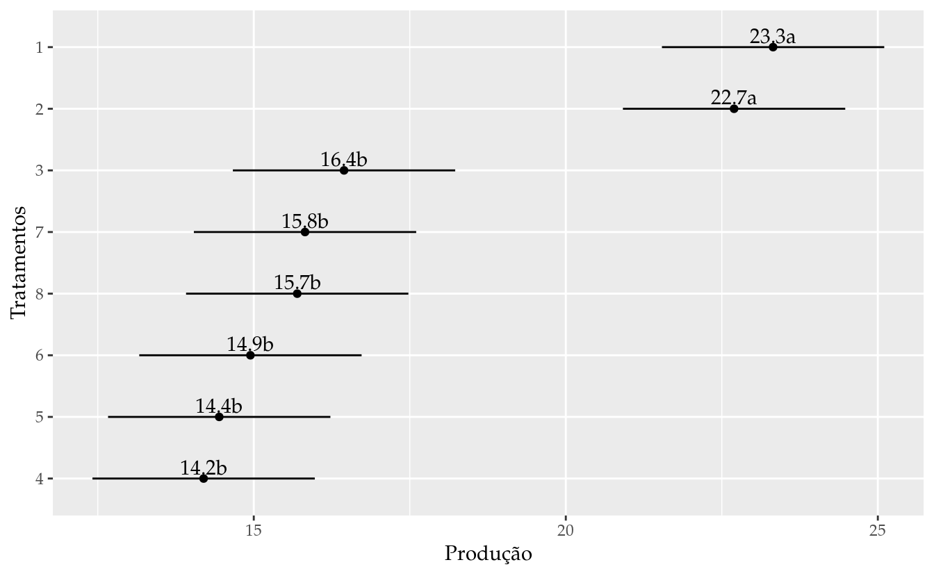
# Gráfico com médias e intervalos para os contrastes.
mmc <- mmc(model = m0,
           linfct = all_pairwise(L, collapse = "-"),
           focus = "trat")
plot(mmc)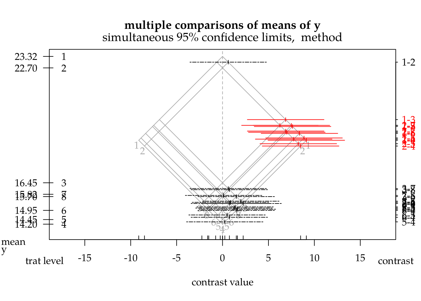
ATTENTION: a HH::mmc() pode demorar bastante quando o número de tratamentos for grande por causa das contas necessárias para obter os intervalos de confiança de cobertura global.
14.1.2 Modelo de efeitos aleatórios
# Modelo de efeitos aleatórios.
mm0 <- lmer(y ~ (1 | rept) + (1 | rept:bloc) + trat,
            data = da)

# Quadro de testes de hipótese para os termos de efeito fixo.
anova(mm0)
## Type III Analysis of Variance Table with Satterthwaite's method
## Sum Sq Mean Sq NumDF DenDF F value Pr(>F)
## trat 564.28 80.611 7 38.768 27.679 3.331e-13 ***
## ---
## Signif. codes: 0 '***' 0.001 '**' 0.01 '*' 0.05 '.' 0.1 ' ' 1# Médias marginais ajustadas.
emm <- emmeans(mm0, specs = ~trat)
emm## trat emmean SE df lower.CL upper.CL
## 1 23.1 0.889 27.1 21.3 24.9
## 2 23.2 0.889 27.1 21.4 25.0
## 3 16.4 0.889 27.1 14.6 18.3
## 4 14.5 0.889 27.1 12.6 16.3
## 5 14.2 0.889 27.1 12.4 16.1
## 6 14.8 0.889 27.1 13.0 16.6
## 7 15.5 0.889 27.1 13.7 17.4
## 8 15.8 0.889 27.1 14.0 17.6
##
## Degrees-of-freedom method: kenward-roger
## Confidence level used: 0.95grid <- attr(emm, "grid")
L <- attr(emm, "linfct")
rownames(L) <- grid[[1]]
# Resultados para colocar em gráfico de segmentos.
results_mm0 <- wzRfun::apmc(L,
model = mm0,
focus = "trat",
test = "fdr")
# Gráfico de segmentos para as estimativas intervalares.
ggplot(data = results_mm0,
mapping = aes(x = fit, y = reorder(trat, fit))) +
geom_point() +
geom_errorbarh(mapping = aes(xmin = lwr, xmax = upr),
height = 0) +
geom_text(mapping = aes(label = sprintf("%0.1f%s", fit, cld)),
vjust = 0,
nudge_y = 0.07) +
labs(x = "Produção",
y = "Tratamentos")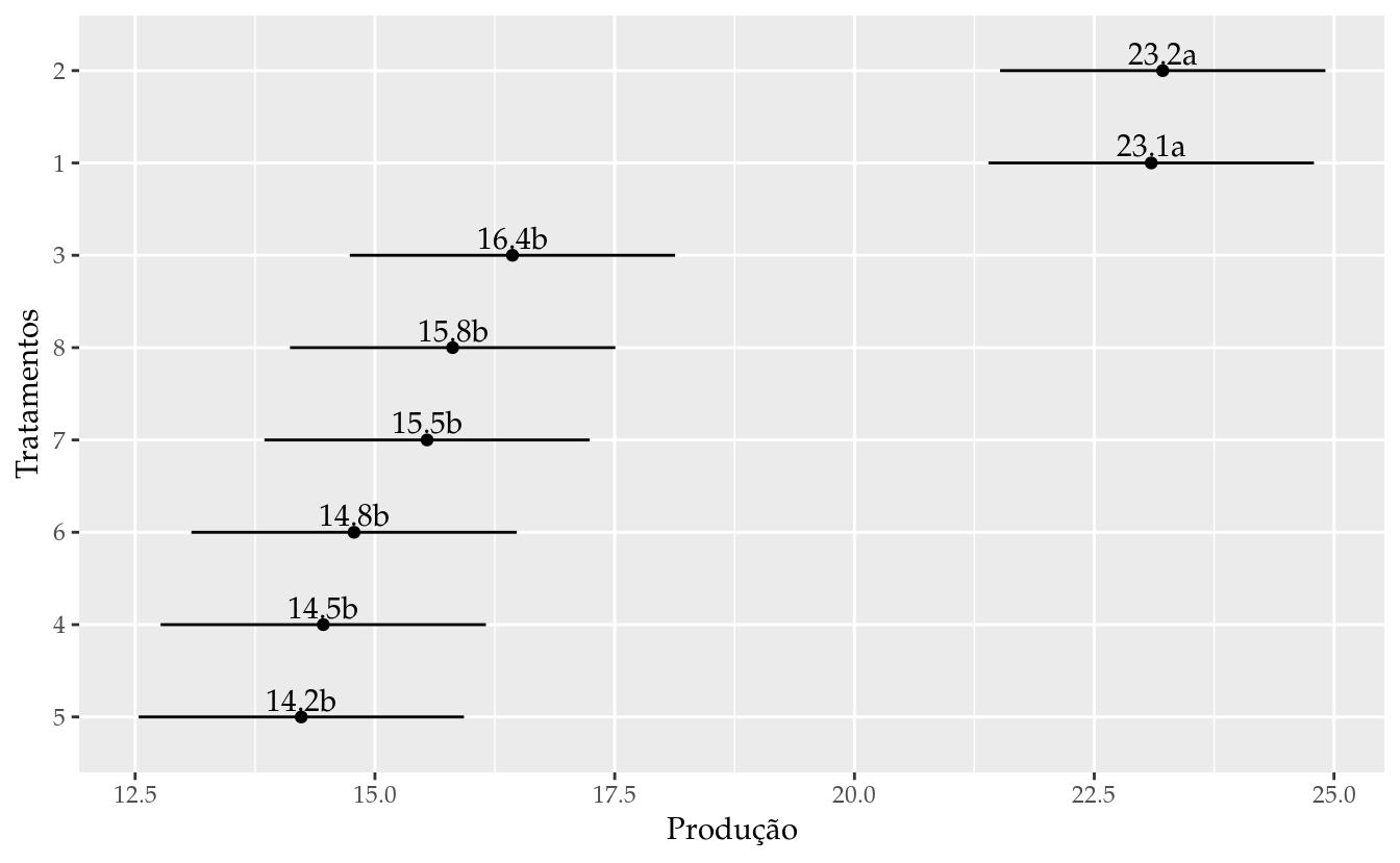
# Gráfico de segmentos para as estimativas intervalares.
results <- bind_rows(list(fixo = results_m0,
aleatorio = results_mm0),
.id = "modelo")
s <- 0.25
pd <- position_dodge(0.25)
ggplot(data = results,
mapping = aes(x = trat,
y = fit,
group = modelo,
color = modelo)) +
geom_point(position = pd) +
geom_errorbar(mapping = aes(ymin = lwr, ymax = upr),
width = 0,
position = pd) +
geom_text(mapping = aes(x = as.integer(trat) +
ifelse(modelo == "fixo", s, -s),
label = sprintf("%0.2f%s", fit, cld)),
position = pd,
hjust = 0.5,
angle = 90,
show.legend = FALSE) +
labs(y = "Produção",
x = "Tratamentos")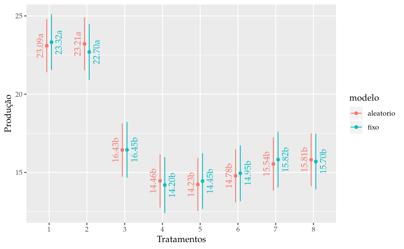
14.2 Bloco incompleto tipo II
14.2.1 Modelo de efeitos fixos
da <- as_tibble(labestData::PimentelTb10.4.1)
str(da)## Classes 'tbl_df', 'tbl' and 'data.frame': 42 obs. of 4 variables:
## $ grup: Factor w/ 3 levels "1","2","3": 1 1 1 1 1 1 1 1 1 1 ...
## $ bloc: Factor w/ 7 levels "1","2","3","4",..: 1 1 2 2 3 3 4 4 5 5 ...
## $ trat: Factor w/ 7 levels "1","2","3","4",..: 1 2 2 3 3 4 4 5 5 6 ...
## $ y : num 3.5 2.8 3.2 3.7 3.5 2.5 2.8 2.7 3 3.2 ...# Repetições, blocos e tratamentos.
with(da, table(bloc, trat, grup)) %>%
addmargins(margin = 1:2) %>%
print.table(zero.print = ".")## , , grup = 1
##
## trat
## bloc 1 2 3 4 5 6 7 Sum
## 1 1 1 . . . . . 2
## 2 . 1 1 . . . . 2
## 3 . . 1 1 . . . 2
## 4 . . . 1 1 . . 2
## 5 . . . . 1 1 . 2
## 6 . . . . . 1 1 2
## 7 1 . . . . . 1 2
## Sum 2 2 2 2 2 2 2 14
##
## , , grup = 2
##
## trat
## bloc 1 2 3 4 5 6 7 Sum
## 1 1 . 1 . . . . 2
## 2 . . 1 . 1 . . 2
## 3 . . . . 1 . 1 2
## 4 . 1 . . . . 1 2
## 5 . 1 . 1 . . . 2
## 6 . . . 1 . 1 . 2
## 7 1 . . . . 1 . 2
## Sum 2 2 2 2 2 2 2 14
##
## , , grup = 3
##
## trat
## bloc 1 2 3 4 5 6 7 Sum
## 1 1 . . 1 . . . 2
## 2 . . . 1 . . 1 2
## 3 . . 1 . . . 1 2
## 4 . . 1 . . 1 . 2
## 5 . 1 . . . 1 . 2
## 6 . 1 . . 1 . . 2
## 7 1 . . . 1 . . 2
## Sum 2 2 2 2 2 2 2 14library(igraph)
edg <- by(data = da$trat,
INDICES = interaction(da$grup, da$bloc),
FUN = combn,
m = 2) %>%
flatten_int()
ghp <- graph(edg, directed = FALSE)
plot(ghp,
layout = layout_in_circle,
edge.curved = FALSE)# Modelo de efeitos fixos.
m0 <- lm(terms(y ~ grup/bloc + trat, keep.order = TRUE),
data = da)
# Checagem dos pressupostos.
par(mfrow = c(2, 2)); plot(m0); layout(1)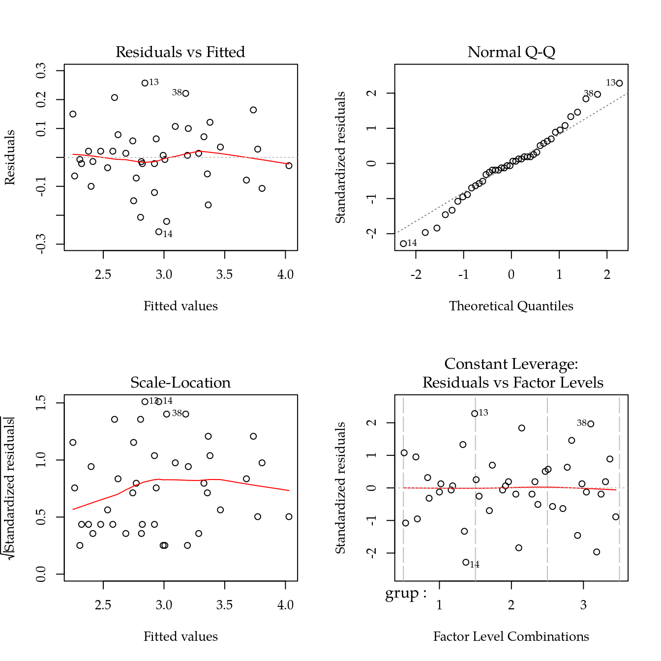
# Quadro de análise de variância (hipóteses sequenciais).
anova(m0)## Analysis of Variance Table
##
## Response: y
## Df Sum Sq Mean Sq F value Pr(>F)
## grup 2 0.0233 0.01167 0.3284 0.7251
## grup:bloc 18 5.3814 0.29897 8.4160 6.859e-05 ***
## trat 6 3.2671 0.54452 15.3284 1.238e-05 ***
## Residuals 15 0.5329 0.03552
## ---
## Signif. codes: 0 '***' 0.001 '**' 0.01 '*' 0.05 '.' 0.1 ' ' 1# Quadro de análise de variância (hipóteses marginais).
Anova(m0)## Anova Table (Type II tests)
##
## Response: y
## Sum Sq Df F value Pr(>F)
## grup 0.0233 2 0.3284 0.725111
## grup:bloc 2.7471 18 4.2962 0.003239 **
## trat 3.2671 6 15.3284 1.238e-05 ***
## Residuals 0.5329 15
## ---
## Signif. codes: 0 '***' 0.001 '**' 0.01 '*' 0.05 '.' 0.1 ' ' 1# Resultado idem ao anterior (o procedimento interno não é).
drop1(m0, scope = . ~ ., test = "F")## Single term deletions
##
## Model:
## y ~ grup/bloc + trat
## Df Sum of Sq RSS AIC F value Pr(>F)
## <none> 0.5329 -129.421
## grup 2 0.6118 1.1447 -101.306 8.6118 0.003231 **
## trat 6 3.2671 3.8000 -58.912 15.3284 1.238e-05 ***
## grup:bloc 18 2.7471 3.2800 -89.093 4.2962 0.003239 **
## ---
## Signif. codes: 0 '***' 0.001 '**' 0.01 '*' 0.05 '.' 0.1 ' ' 1# Médias marginais ajustadas.
emm <- emmeans(m0, specs = ~trat)## NOTE: A nesting structure was detected in the fitted model:
## bloc %in% grupgrid <- attr(emm, "grid")
L <- attr(emm, "linfct")
MASS::fractions(t(L))## [,1] [,2] [,3] [,4] [,5] [,6] [,7]
## (Intercept) 1 1 1 1 1 1 1
## grup2 1/3 1/3 1/3 1/3 1/3 1/3 1/3
## grup3 1/3 1/3 1/3 1/3 1/3 1/3 1/3
## grup1:bloc2 1/21 1/21 1/21 1/21 1/21 1/21 1/21
## grup2:bloc2 1/21 1/21 1/21 1/21 1/21 1/21 1/21
## grup3:bloc2 1/21 1/21 1/21 1/21 1/21 1/21 1/21
## grup1:bloc3 1/21 1/21 1/21 1/21 1/21 1/21 1/21
## grup2:bloc3 1/21 1/21 1/21 1/21 1/21 1/21 1/21
## grup3:bloc3 1/21 1/21 1/21 1/21 1/21 1/21 1/21
## grup1:bloc4 1/21 1/21 1/21 1/21 1/21 1/21 1/21
## grup2:bloc4 1/21 1/21 1/21 1/21 1/21 1/21 1/21
## grup3:bloc4 1/21 1/21 1/21 1/21 1/21 1/21 1/21
## grup1:bloc5 1/21 1/21 1/21 1/21 1/21 1/21 1/21
## grup2:bloc5 1/21 1/21 1/21 1/21 1/21 1/21 1/21
## grup3:bloc5 1/21 1/21 1/21 1/21 1/21 1/21 1/21
## grup1:bloc6 1/21 1/21 1/21 1/21 1/21 1/21 1/21
## grup2:bloc6 1/21 1/21 1/21 1/21 1/21 1/21 1/21
## grup3:bloc6 1/21 1/21 1/21 1/21 1/21 1/21 1/21
## grup1:bloc7 1/21 1/21 1/21 1/21 1/21 1/21 1/21
## grup2:bloc7 1/21 1/21 1/21 1/21 1/21 1/21 1/21
## grup3:bloc7 1/21 1/21 1/21 1/21 1/21 1/21 1/21
## trat2 0 1 0 0 0 0 0
## trat3 0 0 1 0 0 0 0
## trat4 0 0 0 1 0 0 0
## trat5 0 0 0 0 1 0 0
## trat6 0 0 0 0 0 1 0
## trat7 0 0 0 0 0 0 1rownames(L) <- grid[[1]]
# summary(glht(m0, linfct = all_pairwise(L)),
# test = adjusted(type = "fdr"))
# glht0 <- summary(glht(m0, linfct = mcp(trat = "Tukey")),
# test = adjusted(type = "fdr"))
# glht0
# cld(glht0)
# plot(glht0)
results_m0 <- wzRfun::apmc(L,
model = m0,
focus = "trat",
test = "fdr")
results_m0## trat fit lwr upr cld
## 1 1 3.295238 3.086993 3.503483 ab
## 2 2 2.838095 2.629850 3.046340 c
## 3 3 3.552381 3.344136 3.760626 a
## 4 4 2.623810 2.415564 2.832055 cd
## 5 5 2.495238 2.286993 2.703483 d
## 6 6 2.680952 2.472707 2.889197 cd
## 7 7 3.180952 2.972707 3.389197 b# Gráfico de segmentos para as estimativas intervalares.
ggplot(data = results_m0,
mapping = aes(x = fit, y = reorder(trat, fit))) +
geom_point() +
geom_errorbarh(mapping = aes(xmin = lwr, xmax = upr),
height = 0) +
geom_text(mapping = aes(label = sprintf("%0.1f%s", fit, cld)),
vjust = 0,
nudge_y = 0.07) +
labs(x = "Produção",
y = "Tratamentos")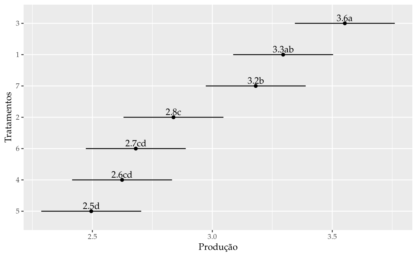
mmc <- mmc(m0,
linfct = all_pairwise(L, collapse = "-"),
focus = "trat")
plot(mmc)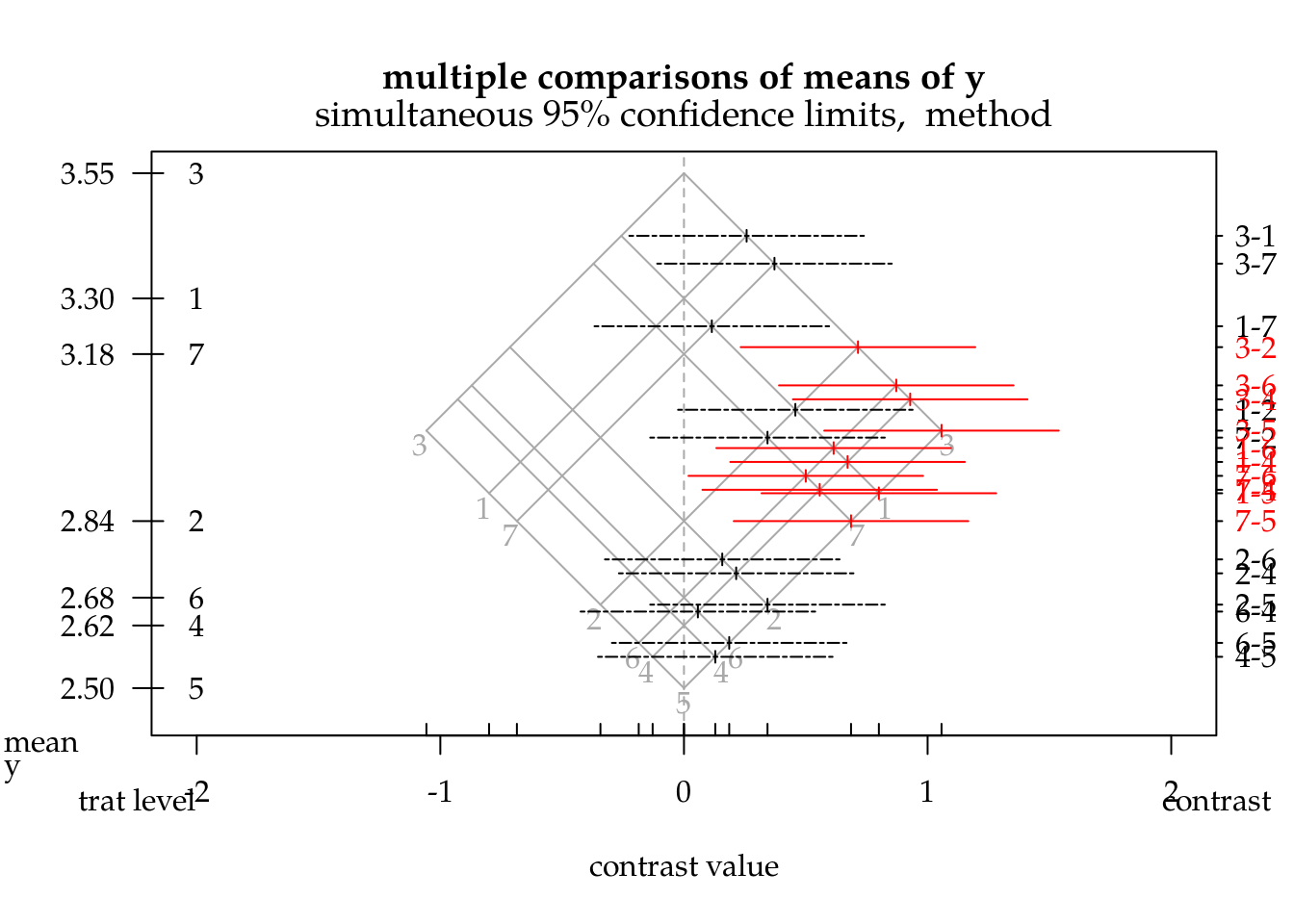
14.2.2 Modelo de efeitos aleatórios
# Modelo de efeitos aleatórios.
mm0 <- lmer(y ~ grup + (1 | grup:bloc) + trat, data = da)
# Quadro de testes de hipótese para os termos de efeito fixo.
anova(mm0)## Type III Analysis of Variance Table with Satterthwaite's method
## Sum Sq Mean Sq NumDF DenDF F value Pr(>F)
## grup 0.0049 0.00243 2 16.862 0.0693 0.9333
## trat 3.7631 0.62718 6 20.065 17.8741 4.34e-07 ***
## ---
## Signif. codes: 0 '***' 0.001 '**' 0.01 '*' 0.05 '.' 0.1 ' ' 1# summary(mm0)
# VarCorr(mm0)
# Médias marginais ajustadas.
emm <- emmeans(mm0, specs = ~trat)
emm
## trat emmean SE df lower.CL upper.CL
## 1 3.29 0.109 31.9 3.06 3.51
## 2 2.86 0.109 31.9 2.63 3.08
## 3 3.59 0.109 31.9 3.37 3.81
## 4 2.60 0.109 31.9 2.38 2.82
## 5 2.53 0.109 31.9 2.31 2.75
## 6 2.68 0.109 31.9 2.45 2.90
## 7 3.13 0.109 31.9 2.91 3.35
##
## Results are averaged over the levels of: grup
## Degrees-of-freedom method: kenward-roger
## Confidence level used: 0.95grid <- attr(emm, "grid")
L <- attr(emm, "linfct")
rownames(L) <- grid[[1]]
# Resultados para colocar em gráfico de segmentos.
results_mm0 <- wzRfun::apmc(L,
model = mm0,
focus = "trat",
test = "fdr")
# Gráfico de segmentos para as estimativas intervalares.
ggplot(data = results_mm0,
mapping = aes(x = fit, y = reorder(trat, fit))) +
geom_point() +
geom_errorbarh(mapping = aes(xmin = lwr, xmax = upr),
height = 0) +
geom_text(mapping = aes(label = sprintf("%0.1f%s", fit, cld)),
vjust = 0,
nudge_y = 0.07) +
labs(x = "Produção",
y = "Tratamentos")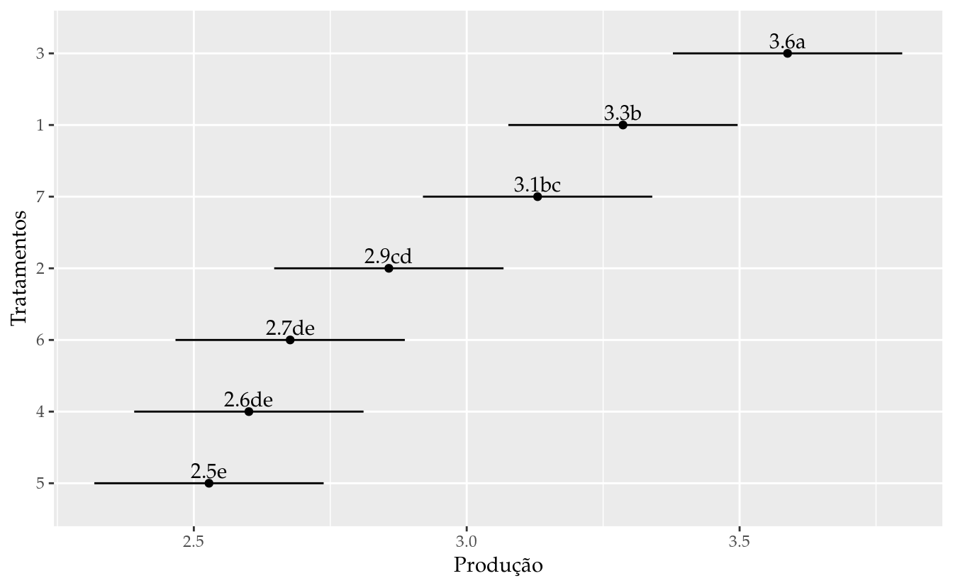
# Gráfico de segmentos para as estimativas intervalares.
results <- bind_rows(list(fixo = results_m0,
                          aleatorio = results_mm0),
                     .id = "modelo")

s <- 0.25
pd <- position_dodge(0.25)
ggplot(data = results,
       mapping = aes(x = trat,
                     y = fit,
                     group = modelo,
                     color = modelo)) +
    geom_point(position = pd) +
    geom_errorbar(mapping = aes(ymin = lwr, ymax = upr),
                  width = 0,
                  position = pd) +
    geom_text(mapping = aes(x = as.integer(trat) +
                                ifelse(modelo == "fixo", s, -s),
                            label = sprintf("%0.2f%s", fit, cld)),
              position = pd,
              hjust = 0.5,
              angle = 90,
              show.legend = FALSE) +
    labs(y = "Produção",
         x = "Tratamentos")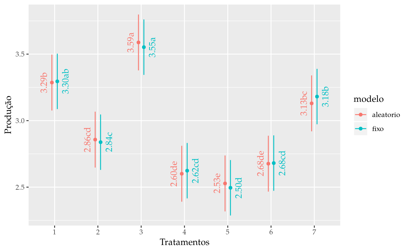
Referências Bibliográficas
PIMENTEL-GOMES, F. Curso de estatística experimental. 15th ed. Piracicaba, SP: FEALQ, 2009.
Manual de Planejamento e Análise de Experimentos com R
Walmes Marques Zeviani