Capítulo 4 Delineamento de Quadrado Latino
4.1 Motivação
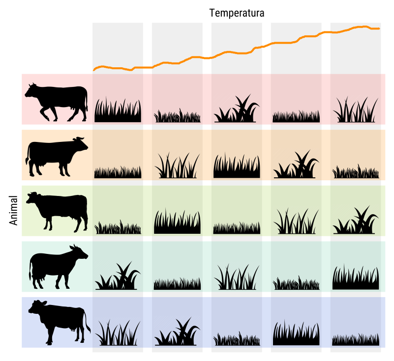
Figura 4.1: Ilustração de um experimento em delineamento quadrado latino 5 \(\times\) 5 para estudar o efeito de 5 tipos de grama no ganho de peso de animais. O quadrado latino está blocando o efeito de animal (linhas) e o efeito ambiental (colunas).
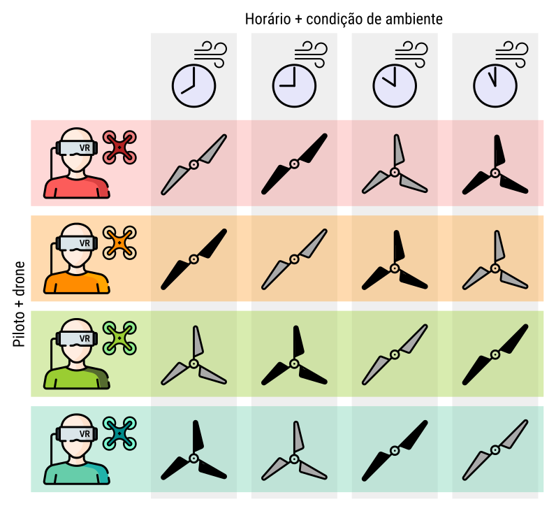
Figura 4.2: Ilustração de um experimento em delineamento quadrado latino 4 \(\times\) 4 para estudar o efeito de 2 tipos de materiais usandos para construção das hélices (plástico e fibra de carbono) combinado com o número de pás (2 e 3 pás) em relação ao tempo de vôo. O quadrado latino está blocando o efeito de piloto com equipamento (linhas, e.g. experiência, desgaste) e o das condições de vôo (colunas, e.g. vento, visibilidade).
# ATTENTION: Limpa espaço de trabalho.
rm(list = objects())

# Carrega pacotes.
library(agricolae) # HSD.test()
library(car)       # linearHypothesis(), Anova()
library(multcomp)  # glht()
library(emmeans)   # emmeans()
library(tidyverse)

# Carrega funções.
source("mpaer_functions.R")
4.2 Variável resposta contínua
da <- labestData::PimentelEg6.2
str(da)
## 'data.frame': 25 obs. of 4 variables:
## $ linha : Factor w/ 5 levels "1","2","3","4",..: 1 2 3 4 5 1 2 3 4 5 ...
## $ coluna: Factor w/ 5 levels "1","2","3","4",..: 1 1 1 1 1 2 2 2 2 2 ...
## $ varied: Factor w/ 5 levels "A","B","C","D",..: 4 3 5 2 1 1 5 2 4 3 ...
## $ prod : int 432 724 489 494 515 518 478 384 500 660 ...# Vendo o quadrado no plano.
reshape2::dcast(da, linha ~ coluna, value.var = "varied")## linha 1 2 3 4 5
## 1 1 D A B C E
## 2 2 C E A B D
## 3 3 E B C D A
## 4 4 B D E A C
## 5 5 A C D E Breshape2::dcast(da, linha ~ coluna, value.var = "prod")## linha 1 2 3 4 5
## 1 1 432 518 458 583 331
## 2 2 724 478 524 550 400
## 3 3 489 384 556 297 420
## 4 4 494 500 313 486 501
## 5 5 515 660 438 394 318# Tem registros perdidos?
sum(is.na(da$prod))## [1] 0# Análise exploratória.
ggplot(data = da,
mapping = aes(x = reorder(varied, prod),
y = prod,
color = linha,
shape = coluna)) +
geom_point() +
stat_summary(mapping = aes(group = 1),
geom = "line",
fun.y = "mean",
show.legend = FALSE)
gg1 <-
    ggplot(data = da,
           mapping = aes(x = coluna,
                         y = linha,
                         fill = varied)) +
    geom_tile() +
    geom_text(mapping = aes(label = sprintf("%s\n%d", varied, prod))) +
    coord_equal()

gg2 <-
    ggplot(data = da,
           mapping = aes(x = coluna,
                         y = linha,
                         fill = prod)) +
    geom_tile() +
    geom_text(mapping = aes(label = sprintf("%s\n%d", varied, prod))) +
    scale_fill_distiller(palette = "Greens", direction = 1) +
    coord_equal()

gridExtra::grid.arrange(gg1, gg2, nrow = 1)
gridExtra::grid.arrange(
               ggplot(data = da,
                      mapping = aes(x = linha, y = prod)) +
               geom_col(),
               ggplot(data = da,
                      mapping = aes(x = coluna, y = prod)) +
               geom_col(),
               ggplot(data = da,
                      mapping = aes(x = varied, y = prod)) +
               geom_col(),
               nrow = 1)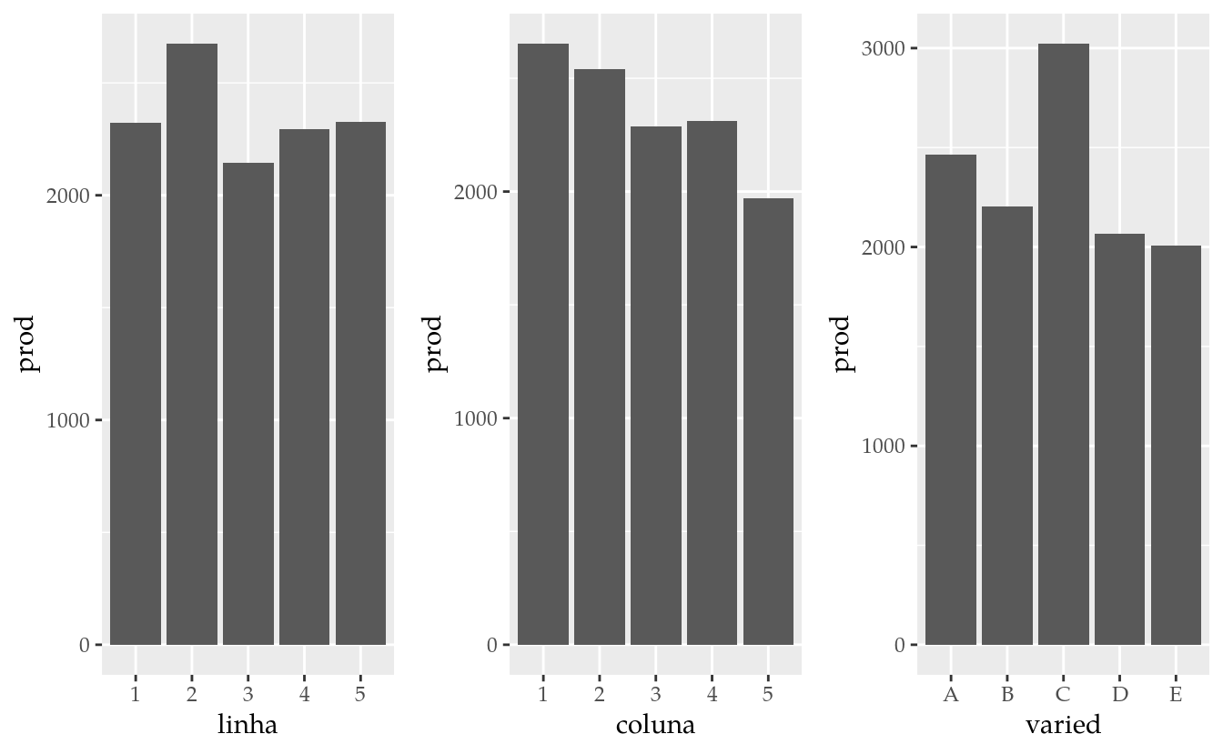
O modelo estatístico para esse experimento é \[ \begin{aligned} Y|i, j, k &\sim \text{Normal}(\mu_{ijk}, \sigma^2) \\ \mu_{ijk} &= \mu + \alpha_i + \beta_j + \tau_k \end{aligned} \] em que \(\alpha_i\) é o efeito da linha \(i\), \(\beta_j\) é o efeito da coluna \(j\) e \(\tau_j\) o efeito da variedade \(j\) sobre a variável resposta \(Y\), \(\mu\) é a média de \(Y\) na ausência do efeito dos termos mencionados, \(\mu_{ijk}\) é a média para as observações de procedência \(ijk\) e \(\sigma^2\) é a variância das observações ao redor desse valor médio.
m0 <- lm(prod ~ linha + coluna + varied, data = da)

# Diganóstico dos resíduos.
par(mfrow = c(2, 2))
plot(m0)
layout(1)

# Quadro de análise de variância.
# anova(m0)
Anova(m0)
## Anova Table (Type II tests)
##
## Response: prod
## Sum Sq Df F value Pr(>F)
## linha 30481 4 2.6804 0.0831343 .
## coluna 55641 4 4.8930 0.0142293 *
## varied 137488 4 12.0905 0.0003585 ***
## Residuals 34115 12
## ---
## Signif. codes: 0 '***' 0.001 '**' 0.01 '*' 0.05 '.' 0.1 ' ' 1# Estimativas dos efeitos e medidas de ajuste.
summary(m0)##
## Call:
## lm(formula = prod ~ linha + coluna + varied, data = da)
##
## Residuals:
## Min 1Q Median 3Q Max
## -66.56 -25.16 -1.56 23.24 69.04
##
## Coefficients:
## Estimate Std. Error t value Pr(>|t|)
## (Intercept) 546.76 38.45 14.220 7.14e-09 ***
## linha2 70.80 33.72 2.100 0.05759 .
## linha3 -35.20 33.72 -1.044 0.31713
## linha4 -5.60 33.72 -0.166 0.87087
## linha5 0.60 33.72 0.018 0.98610
## coluna2 -22.80 33.72 -0.676 0.51178
## coluna3 -73.00 33.72 -2.165 0.05127 .
## coluna4 -68.80 33.72 -2.040 0.06397 .
## coluna5 -136.80 33.72 -4.057 0.00159 **
## variedB -51.80 33.72 -1.536 0.15045
## variedC 112.20 33.72 3.327 0.00603 **
## variedD -79.20 33.72 -2.349 0.03680 *
## variedE -91.60 33.72 -2.716 0.01873 *
## ---
## Signif. codes: 0 '***' 0.001 '**' 0.01 '*' 0.05 '.' 0.1 ' ' 1
##
## Residual standard error: 53.32 on 12 degrees of freedom
## Multiple R-squared: 0.8676, Adjusted R-squared: 0.7353
## F-statistic: 6.555 on 12 and 12 DF, p-value: 0.001366# Comparações múltiplas.
# Médias marginais ajustadas.
emm <- emmeans(m0, specs = ~varied)
emm## varied emmean SE df lower.CL upper.CL
## A 493 23.8 12 441 545
## B 441 23.8 12 389 493
## C 605 23.8 12 553 657
## D 413 23.8 12 361 465
## E 401 23.8 12 349 453
##
## Results are averaged over the levels of: linha, coluna
## Confidence level used: 0.95grid <- attr(emm, "grid")
L <- attr(emm, "linfct")
rownames(L) <- grid[[1]]
MASS::fractions(L)## (Intercept) linha2 linha3 linha4 linha5 coluna2 coluna3 coluna4
## A 1 1/5 1/5 1/5 1/5 1/5 1/5 1/5
## B 1 1/5 1/5 1/5 1/5 1/5 1/5 1/5
## C 1 1/5 1/5 1/5 1/5 1/5 1/5 1/5
## D 1 1/5 1/5 1/5 1/5 1/5 1/5 1/5
## E 1 1/5 1/5 1/5 1/5 1/5 1/5 1/5
## coluna5 variedB variedC variedD variedE
## A 1/5 0 0 0 0
## B 1/5 1 0 0 0
## C 1/5 0 1 0 0
## D 1/5 0 0 1 0
## E 1/5 0 0 0 1# Comparações múltiplas, contrastes de Tukey.
# Método de correção de p-valor: single-step.
tk_sgl <- summary(glht(m0, linfct = mcp(varied = "Tukey")),
test = adjusted(type = "single-step"))
tk_sgl##
## Simultaneous Tests for General Linear Hypotheses
##
## Multiple Comparisons of Means: Tukey Contrasts
##
##
## Fit: lm(formula = prod ~ linha + coluna + varied, data = da)
##
## Linear Hypotheses:
## Estimate Std. Error t value Pr(>|t|)
## B - A == 0 -51.80 33.72 -1.536 0.56049
## C - A == 0 112.20 33.72 3.327 0.03937 *
## D - A == 0 -79.20 33.72 -2.349 0.19550
## E - A == 0 -91.60 33.72 -2.716 0.10979
## C - B == 0 164.00 33.72 4.863 0.00295 **
## D - B == 0 -27.40 33.72 -0.813 0.92175
## E - B == 0 -39.80 33.72 -1.180 0.76212
## D - C == 0 -191.40 33.72 -5.676 < 0.001 ***
## E - C == 0 -203.80 33.72 -6.044 < 0.001 ***
## E - D == 0 -12.40 33.72 -0.368 0.99555
## ---
## Signif. codes: 0 '***' 0.001 '**' 0.01 '*' 0.05 '.' 0.1 ' ' 1
## (Adjusted p values reported -- single-step method)# Resumo compacto com letras.
cld(tk_sgl, decreasing = TRUE)## A B C D E
## "b" "b" "a" "b" "b"# Teste HSD de Tukey.
tk_hsd <- HSD.test(m0, trt = "varied")
# Detalhes da aplicação do teste HSD de Tukey.
tk_hsd$parameters## test name.t ntr StudentizedRange alpha
## Tukey varied 5 4.50771 0.05tk_hsd$statistics## MSerror Df Mean CV MSD
## 2842.893 12 470.52 11.33189 107.4858results <- tk_hsd$groups %>%
rownames_to_column("varied")
results <- inner_join(results,
as.data.frame(emm))## Joining, by = "varied"results## varied prod groups emmean SE df lower.CL upper.CL
## 1 C 604.8 a 604.8 23.84489 12 552.8465 656.7535
## 2 A 492.6 b 492.6 23.84489 12 440.6465 544.5535
## 3 B 440.8 b 440.8 23.84489 12 388.8465 492.7535
## 4 D 413.4 b 413.4 23.84489 12 361.4465 465.3535
## 5 E 401.0 b 401.0 23.84489 12 349.0465 452.9535# Gráfico com estimativas, IC e texto.
ggplot(data = results,
mapping = aes(x = reorder(varied, prod), y = prod)) +
geom_point() +
geom_errorbar(mapping = aes(ymin = lower.CL, ymax = upper.CL),
width = 0) +
geom_label(mapping = aes(label = sprintf("%0.1f %s", prod, groups)),
nudge_y = 5,
vjust = 0) +
labs(x = "Variedade", y = "Produção")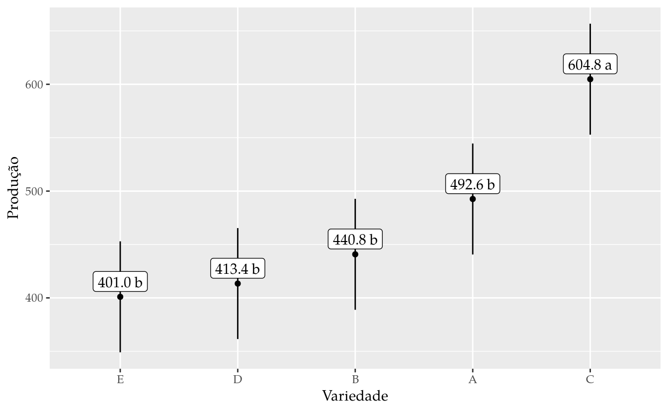
TODO! Colocar teste de Scott Knott.
4.3 Variável resposta de contagem
da <- labestData::ZimmermannTb16.10
str(da)
## 'data.frame': 36 obs. of 5 variables:
## $ linha : Factor w/ 6 levels "1","2","3","4",..: 1 2 3 4 5 6 1 2 3 4 ...
## $ coluna: Factor w/ 6 levels "1","2","3","4",..: 1 1 1 1 1 1 2 2 2 2 ...
## $ trat : Factor w/ 6 levels "1","2","3","4",..: 5 4 3 1 6 2 2 6 4 5 ...
## $ colmos: num 20 17 16 8 4 22 5 4 8 14 ...
## $ posto : num 34 32.5 30.5 15 4 35 7 4 15 29 ...# Análise exploratória.
ggplot(data = da,
mapping = aes(x = reorder(trat, colmos),
y = colmos,
color = linha,
shape = coluna)) +
geom_point() +
stat_summary(mapping = aes(group = 1),
geom = "line",
fun.y = "mean",
show.legend = FALSE)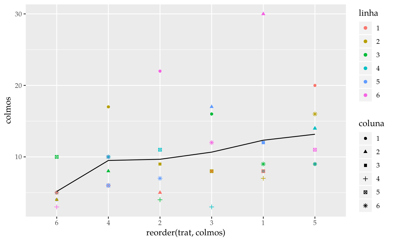
gg1 <-
    ggplot(data = da,
           mapping = aes(x = coluna,
                         y = linha,
                         fill = trat)) +
    geom_tile(show.legend = FALSE) +
    geom_text(mapping = aes(label = sprintf("[%s]\n%d",
                                            trat,
                                            colmos)),
              size = 3) +
    coord_equal()

gg2 <-
    ggplot(data = da,
           mapping = aes(x = coluna,
                         y = linha,
                         fill = colmos)) +
    geom_tile(show.legend = FALSE) +
    geom_text(mapping = aes(label = sprintf("[%s]\n%d",
                                            trat,
                                            colmos)),
              size = 3) +
    scale_fill_distiller(palette = "Greens", direction = 1) +
    coord_equal()

gridExtra::grid.arrange(gg1, gg2, nrow = 1)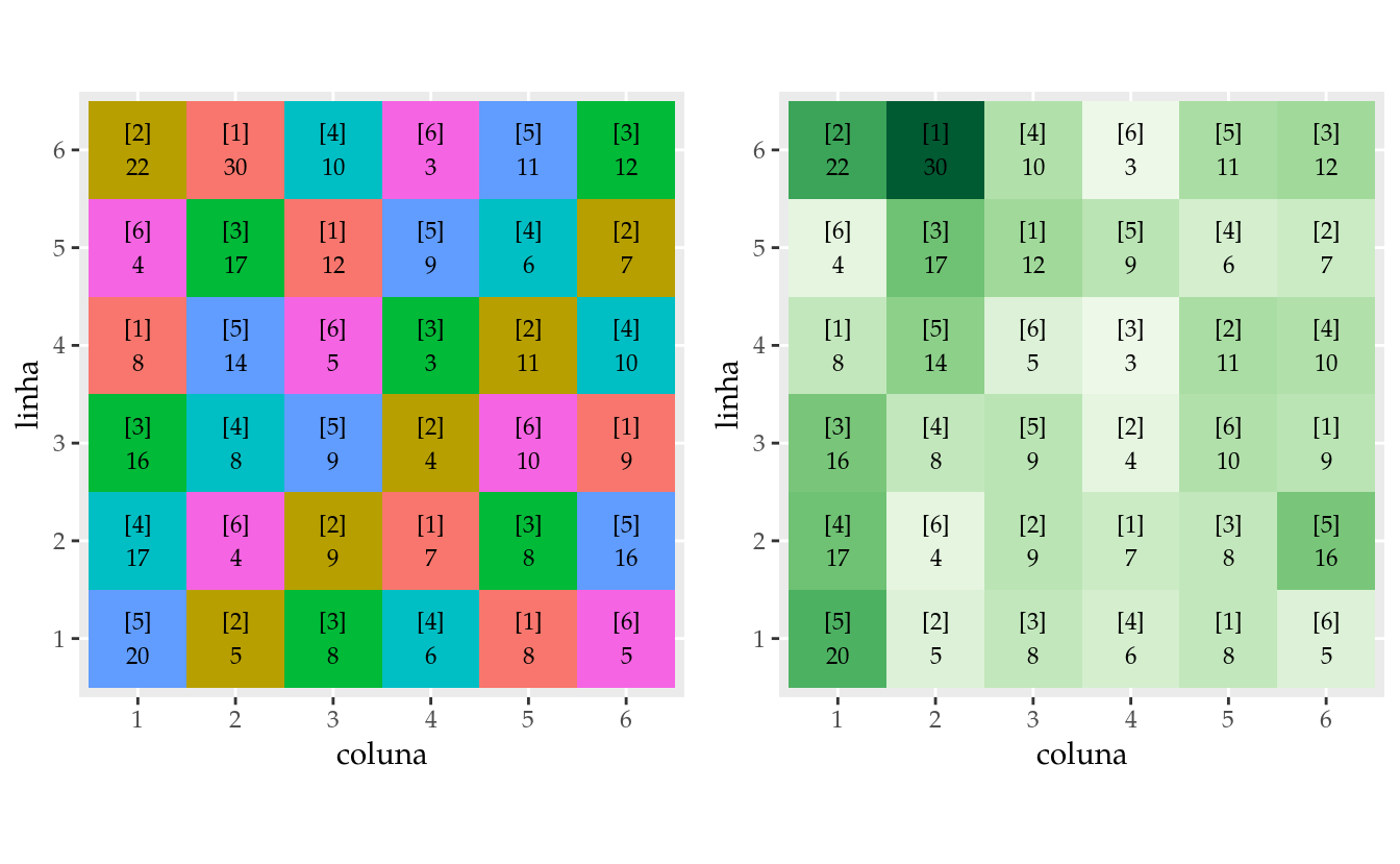
m0 <- lm(colmos ~ linha + coluna + trat,
         data = da)

# Diganóstico dos resíduos.
par(mfrow = c(2, 2))
plot(m0)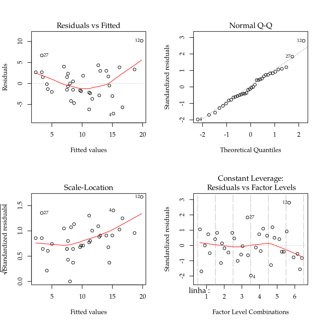
layout(1)MASS::boxcox(m0)
abline(v = 0, col = "red")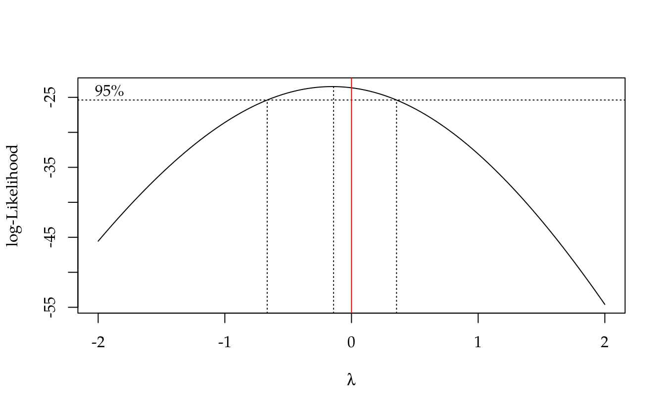
# Análise com modelo linear generalizado.
m0 <- glm(colmos ~ linha + coluna + trat,
          data = da,
          family = quasipoisson)

# Diganóstico dos resíduos.
par(mfrow = c(2, 2))
plot(m0)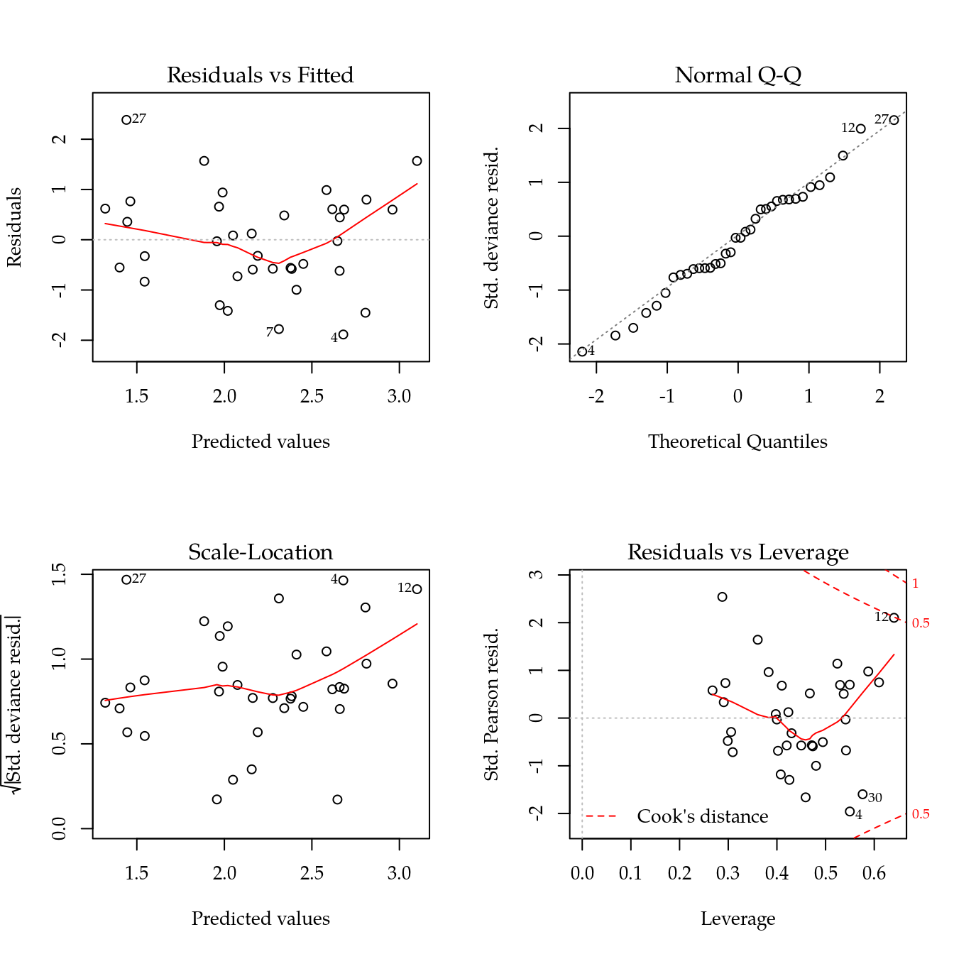
layout(1)

# Quadro de análise de variância.
# anova(m0, test = "F")
# drop1(m0, test = "F")
Anova(m0, test.statistic = "F")
## Analysis of Deviance Table (Type II tests)
##
## Response: colmos
## Error estimate based on Pearson residuals
##
## Sum Sq Df F value Pr(>F)
## linha 13.717 5 1.5953 0.20700
## coluna 31.890 5 3.7089 0.01545 *
## trat 25.095 5 2.9187 0.03882 *
## Residuals 34.393 20
## ---
## Signif. codes: 0 '***' 0.001 '**' 0.01 '*' 0.05 '.' 0.1 ' ' 1# Estimativas dos efeitos e medidas de ajuste.
summary(m0)##
## Call:
## glm(formula = colmos ~ linha + coluna + trat, family = quasipoisson,
## data = da)
##
## Deviance Residuals:
## Min 1Q Median 3Q Max
## -1.88545 -0.59977 -0.02819 0.61018 2.38466
##
## Coefficients:
## Estimate Std. Error t value Pr(>|t|)
## (Intercept) 2.71423 0.26116 10.393 1.65e-09 ***
## linha2 0.23219 0.25203 0.921 0.36789
## linha3 0.09138 0.25699 0.356 0.72587
## linha4 -0.03471 0.26078 -0.133 0.89543
## linha5 0.14659 0.25856 0.567 0.57707
## linha6 0.51768 0.23222 2.229 0.03742 *
## coluna2 -0.13126 0.20738 -0.633 0.53395
## coluna3 -0.51876 0.23095 -2.246 0.03614 *
## coluna4 -0.98911 0.27372 -3.614 0.00173 **
## coluna5 -0.52364 0.23017 -2.275 0.03406 *
## coluna6 -0.42738 0.22410 -1.907 0.07098 .
## trat2 -0.27135 0.23280 -1.166 0.25748
## trat3 -0.14607 0.22725 -0.643 0.52766
## trat4 -0.26224 0.23475 -1.117 0.27720
## trat5 0.09777 0.21509 0.455 0.65431
## trat6 -0.84142 0.28385 -2.964 0.00767 **
## ---
## Signif. codes: 0 '***' 0.001 '**' 0.01 '*' 0.05 '.' 0.1 ' ' 1
##
## (Dispersion parameter for quasipoisson family taken to be 1.719689)
##
## Null deviance: 105.922 on 35 degrees of freedom
## Residual deviance: 33.373 on 20 degrees of freedom
## AIC: NA
##
## Number of Fisher Scoring iterations: 4# Comparações múltiplas.
# Médias marginais ajustadas.
emmeans(m0, specs = ~trat, transform = "response")## trat rate SE df asymp.LCL asymp.UCL
## 1 12.27 1.90 Inf 8.56 15.99
## 2 9.36 1.63 Inf 6.16 12.55
## 3 10.60 1.76 Inf 7.16 14.05
## 4 9.44 1.66 Inf 6.19 12.69
## 5 13.53 2.03 Inf 9.56 17.50
## 6 5.29 1.25 Inf 2.83 7.75
##
## Results are averaged over the levels of: linha, coluna
## Confidence level used: 0.95# emmeans(m0, specs = ~trat, transform = "unlink") # Igual.
# emmeans(m0, specs = ~trat, transform = "mu") # Igual.
emm <- emmeans(m0, specs = ~trat)
emm## trat emmean SE df asymp.LCL asymp.UCL
## 1 2.44 0.157 Inf 2.13 2.75
## 2 2.17 0.178 Inf 1.82 2.52
## 3 2.30 0.168 Inf 1.97 2.62
## 4 2.18 0.178 Inf 1.83 2.53
## 5 2.54 0.150 Inf 2.25 2.83
## 6 1.60 0.238 Inf 1.13 2.07
##
## Results are averaged over the levels of: linha, coluna
## Results are given on the log (not the response) scale.
## Confidence level used: 0.95emm %>%
as.data.frame() %>%
mutate_at(c("emmean", "asymp.LCL", "asymp.UCL"),
m0$family$linkinv)## trat emmean SE df asymp.LCL asymp.UCL
## 1 1 11.489082 0.1566962 Inf 8.450944 15.619437
## 2 2 8.758667 0.1779058 Inf 6.180226 12.412855
## 3 3 9.927643 0.1680897 Inf 7.141147 13.801437
## 4 4 8.838844 0.1778836 Inf 6.237070 12.525939
## 5 5 12.669178 0.1498617 Inf 9.444652 16.994598
## 6 6 4.952933 0.2376598 Inf 3.108609 7.891488# DANGER FIXME: o que a `transform = "response"` está fazendo não é
# passar o inverso da função de ligação. O que está sendo feito então?
grid <- attr(emm, "grid")
L <- attr(emm, "linfct")
rownames(L) <- grid[[1]]
MASS::fractions(t(L))## 1 2 3 4 5 6
## (Intercept) 1 1 1 1 1 1
## linha2 1/6 1/6 1/6 1/6 1/6 1/6
## linha3 1/6 1/6 1/6 1/6 1/6 1/6
## linha4 1/6 1/6 1/6 1/6 1/6 1/6
## linha5 1/6 1/6 1/6 1/6 1/6 1/6
## linha6 1/6 1/6 1/6 1/6 1/6 1/6
## coluna2 1/6 1/6 1/6 1/6 1/6 1/6
## coluna3 1/6 1/6 1/6 1/6 1/6 1/6
## coluna4 1/6 1/6 1/6 1/6 1/6 1/6
## coluna5 1/6 1/6 1/6 1/6 1/6 1/6
## coluna6 1/6 1/6 1/6 1/6 1/6 1/6
## trat2 0 1 0 0 0 0
## trat3 0 0 1 0 0 0
## trat4 0 0 0 1 0 0
## trat5 0 0 0 0 1 0
## trat6 0 0 0 0 0 1# Comparações múltiplas, contrastes de Tukey.
# Método de correção de p-valor: single-step.
tk_sgl <- summary(glht(m0, linfct = mcp(trat = "Tukey")),
test = adjusted(type = "single-step"))
tk_sgl##
## Simultaneous Tests for General Linear Hypotheses
##
## Multiple Comparisons of Means: Tukey Contrasts
##
##
## Fit: glm(formula = colmos ~ linha + coluna + trat, family = quasipoisson,
## data = da)
##
## Linear Hypotheses:
## Estimate Std. Error z value Pr(>|z|)
## 2 - 1 == 0 -0.271353 0.232799 -1.166 0.8512
## 3 - 1 == 0 -0.146074 0.227249 -0.643 0.9875
## 4 - 1 == 0 -0.262241 0.234753 -1.117 0.8727
## 5 - 1 == 0 0.097775 0.215091 0.455 0.9975
## 6 - 1 == 0 -0.841417 0.283849 -2.964 0.0352 *
## 3 - 2 == 0 0.125279 0.241259 0.519 0.9954
## 4 - 2 == 0 0.009112 0.248187 0.037 1.0000
## 5 - 2 == 0 0.369128 0.230062 1.604 0.5919
## 6 - 2 == 0 -0.570064 0.294950 -1.933 0.3781
## 4 - 3 == 0 -0.116167 0.241506 -0.481 0.9968
## 5 - 3 == 0 0.243849 0.224111 1.088 0.8847
## 6 - 3 == 0 -0.695343 0.288885 -2.407 0.1513
## 5 - 4 == 0 0.360016 0.231370 1.556 0.6241
## 6 - 4 == 0 -0.579176 0.294539 -1.966 0.3580
## 6 - 5 == 0 -0.939192 0.280995 -3.342 0.0106 *
## ---
## Signif. codes: 0 '***' 0.001 '**' 0.01 '*' 0.05 '.' 0.1 ' ' 1
## (Adjusted p values reported -- single-step method)# Resumo compacto com letras.
cld(tk_sgl, decreasing = TRUE)## 1 2 3 4 5 6
## "a" "ab" "ab" "ab" "a" "b"results <- wzRfun::apmc(X = L,
model = m0,
focus = "trat",
test = "single-step") %>%
mutate_at(c("fit", "lwr", "upr"),
m0$family$linkinv)
# Gráfico com estimativas, IC e texto.
ggplot(data = results,
mapping = aes(x = reorder(trat, fit), y = fit)) +
geom_point() +
geom_errorbar(mapping = aes(ymin = lwr, ymax = upr),
width = 0) +
geom_label(mapping = aes(label = sprintf("%0.2f %s", fit, cld)),
nudge_y = 0.25,
vjust = 0) +
labs(x = "Tratamento", y = "Número de colmos atacados")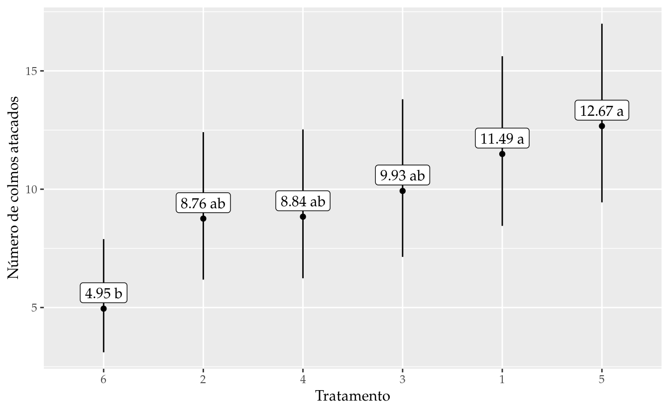
4.4 Variável resposta de proporção amostral
da <- labestData::ZimmermannTb5.11
str(da)
## 'data.frame': 484 obs. of 5 variables:
## $ linha : Factor w/ 11 levels "1","2","3","4",..: 1 2 3 4 5 6 7 8 9 10 ...
## $ coluna : Factor w/ 11 levels "1","2","3","4",..: 1 1 1 1 1 1 1 1 1 1 ...
## $ inset : Factor w/ 11 levels "1","2","3","4",..: 2 6 3 7 4 11 10 5 1 8 ...
## $ amostra: int 1 1 1 1 1 1 1 1 1 1 ...
## $ prop : num 0.9 0.737 0.918 1 0.862 ...# Análise exploratória.
ggplot(data = da,
mapping = aes(x = reorder(inset, prop),
y = prop,
color = linha,
size = coluna)) +
geom_jitter(width = 0.15, show.legend = FALSE) +
stat_summary(mapping = aes(group = 1),
geom = "line",
fun.y = "mean",
show.legend = FALSE)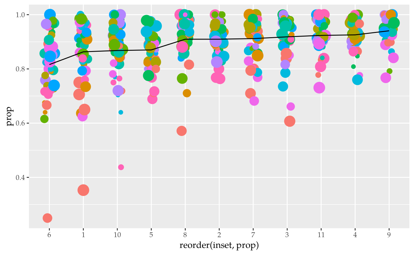
db <- da %>%
    group_by(linha, coluna, inset) %>%
    summarise_at("prop", "mean")

gg1 <-
    ggplot(data = db,
           mapping = aes(x = coluna,
                         y = linha,
                         fill = inset)) +
    geom_tile(show.legend = FALSE) +
    geom_text(mapping = aes(label = sprintf("%s\n%0.2f",
                                            inset,
                                            prop)),
              size = 2) +
    coord_equal()

gg2 <-
    ggplot(data = db,
           mapping = aes(x = coluna,
                         y = linha,
                         fill = prop)) +
    geom_tile(show.legend = FALSE) +
    geom_text(mapping = aes(label = sprintf("%s\n%0.2f",
                                            inset,
                                            prop)),
              size = 2) +
    scale_fill_distiller(palette = "Greens", direction = 1) +
    coord_equal()

gridExtra::grid.arrange(gg1, gg2, nrow = 1)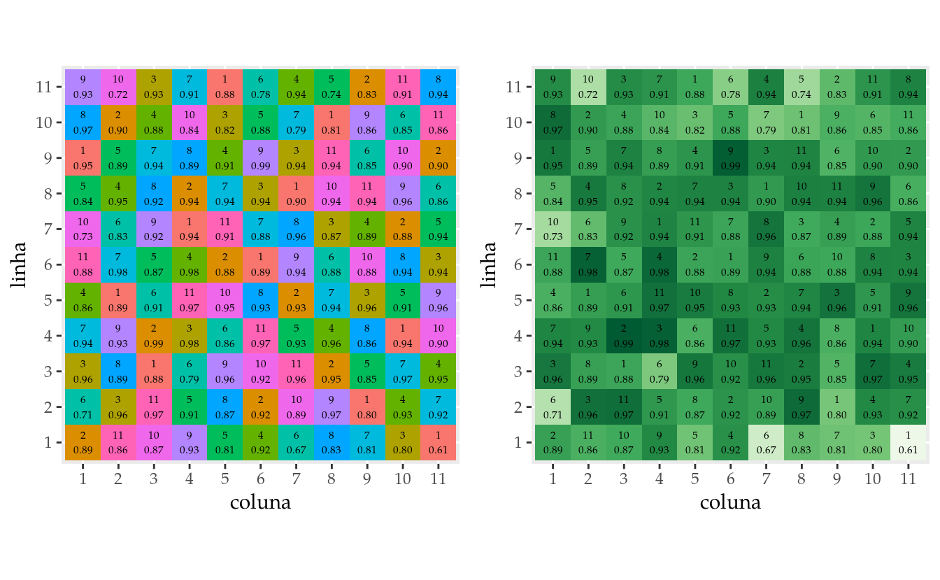
m0 <- lm(prop ~ linha + coluna + inset,
         data = db)

# Diganóstico dos resíduos.
par(mfrow = c(1, 2))
plot(m0, which = 2:3)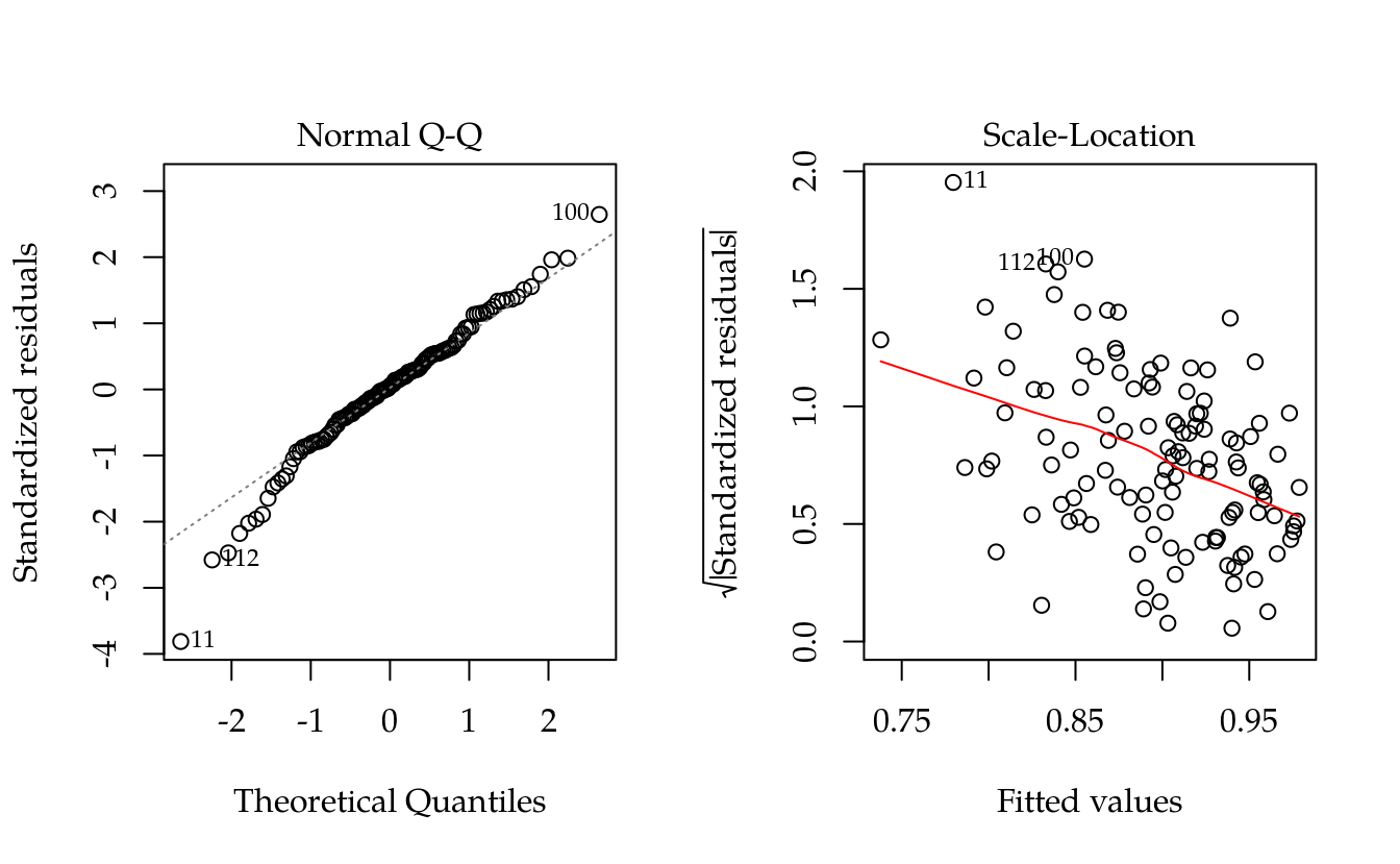
layout(1)

# ATTENTION: Box-Cox não resolve problemas de relação média-variância
# decrescente.

# Modelo para o desfecho complementar.
m0 <- lm(c(1 - prop) ~ linha + coluna + inset,
         data = db)

# Diganóstico dos resíduos.
par(mfrow = c(1, 2))
plot(m0, which = 2:3)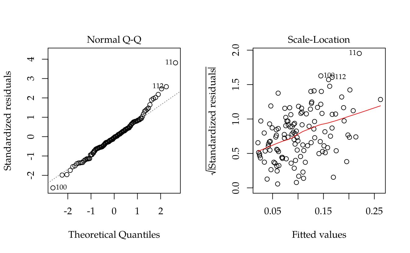
layout(1)

MASS::boxcox(m0)
abline(v = 1/3, col = "red")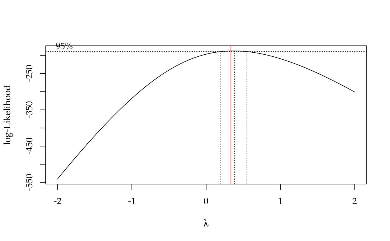
# Transformação arco seno da raíz quadrada da proporção amostral.
db$asinsqrt <- asin(sqrt(db$prop))
m0 <- lm(asinsqrt ~ linha + coluna + inset,
         data = db)

# Diganóstico dos resíduos.
par(mfrow = c(1, 2))
plot(m0, which = 2:3)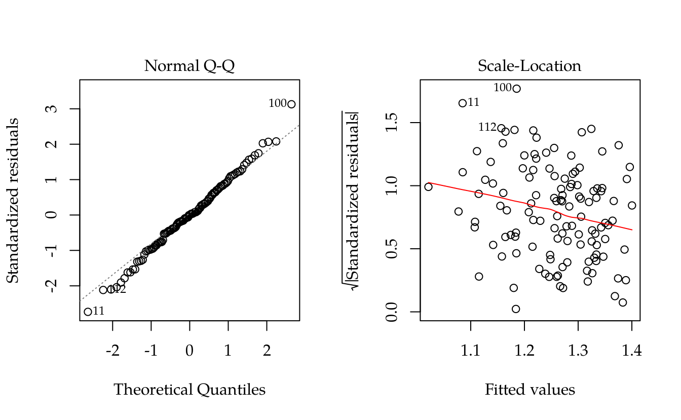
layout(1)

# DISCUSSION: Pressupostos melhor atendidos.

# ATTENTION FIXME: não sabemos o denominador dessa binomial! E pode ser
# que esse `n` seja variável em função da abundância de hastes em cada
# unidade experimental.

# Análise com modelo linear generalizado.
size <- 1
m0 <- glm(cbind(size * prop, size - size * prop) ~
              linha + coluna + inset,
          data = db,
          family = quasibinomial)

# TIP: as inferências são invariantes ao valor do `size` para
# quasibinomial. O parâmetro de dispersão absorve o `size`.
size <- 100
m0 <- glm(cbind(size * prop, size - size * prop) ~ linha + coluna + inset,
          data = db,
          family = quasibinomial)

# Var(Y|.) = \phi * p * (1 - p).

# Diganóstico dos resíduos.
par(mfrow = c(1, 2))
plot(m0, which = 2:3)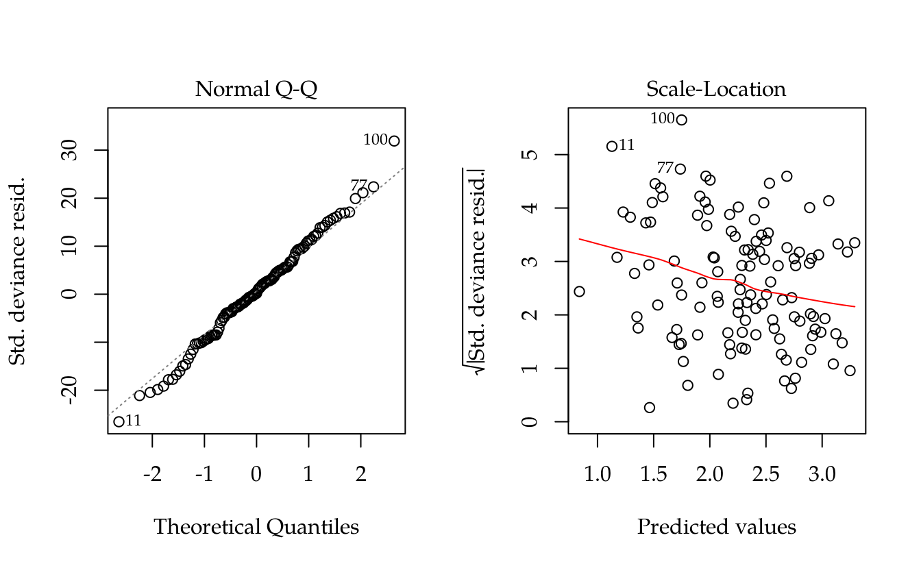
layout(1)

# Quadro de análise de variância.
# anova(m0, test = "F")
# drop1(m0, test = "F")
Anova(m0, test.statistic = "F")
## Analysis of Deviance Table (Type II tests)
##
## Response: cbind(size * prop, size - size * prop)
## Error estimate based on Pearson residuals
##
## Sum Sq Df F value Pr(>F)
## linha 145.289 10 6.5060 1.735e-07 ***
## coluna 32.285 10 1.4457 0.1735
## inset 158.438 10 7.0949 3.910e-08 ***
## Residuals 200.982 90
## ---
## Signif. codes: 0 '***' 0.001 '**' 0.01 '*' 0.05 '.' 0.1 ' ' 1# Estimativas dos efeitos e medidas de ajuste.
summary(m0)##
## Call:
## glm(formula = cbind(size * prop, size - size * prop) ~ linha +
## coluna + inset, family = quasibinomial, data = db)
##
## Deviance Residuals:
## Min 1Q Median 3Q Max
## -3.1151 -0.6806 0.0222 0.8498 3.9362
##
## Coefficients:
## Estimate Std. Error t value Pr(>|t|)
## (Intercept) 0.98666 0.22113 4.462 2.34e-05 ***
## linha2 0.68103 0.19177 3.551 0.000612 ***
## linha3 0.85798 0.20210 4.245 5.30e-05 ***
## linha4 1.14410 0.21680 5.277 9.00e-07 ***
## linha5 1.03704 0.21156 4.902 4.18e-06 ***
## linha6 0.87689 0.20209 4.339 3.73e-05 ***
## linha7 0.55864 0.18714 2.985 0.003649 **
## linha8 0.99211 0.20733 4.785 6.65e-06 ***
## linha9 0.97857 0.20648 4.739 7.98e-06 ***
## linha10 0.28127 0.17737 1.586 0.116293
## linha11 0.34897 0.17919 1.947 0.054596 .
## coluna2 0.16076 0.20388 0.789 0.432457
## coluna3 0.42682 0.21766 1.961 0.052978 .
## coluna4 0.44254 0.21694 2.040 0.044287 *
## coluna5 0.13662 0.20418 0.669 0.505129
## coluna6 0.39098 0.21437 1.824 0.071494 .
## coluna7 0.22780 0.20684 1.101 0.273691
## coluna8 0.19574 0.20576 0.951 0.343998
## coluna9 -0.13141 0.19426 -0.676 0.500483
## coluna10 0.33594 0.21262 1.580 0.117619
## coluna11 0.14194 0.20361 0.697 0.487503
## inset2 0.50115 0.20832 2.406 0.018189 *
## inset3 0.56819 0.21284 2.670 0.009010 **
## inset4 0.66213 0.21867 3.028 0.003212 **
## inset5 0.05070 0.18983 0.267 0.790019
## inset6 -0.37568 0.17832 -2.107 0.037918 *
## inset7 0.50668 0.20921 2.422 0.017445 *
## inset8 0.48097 0.20716 2.322 0.022506 *
## inset9 0.93382 0.23402 3.990 0.000134 ***
## inset10 0.01659 0.18972 0.087 0.930501
## inset11 0.65643 0.21709 3.024 0.003252 **
## ---
## Signif. codes: 0 '***' 0.001 '**' 0.01 '*' 0.05 '.' 0.1 ' ' 1
##
## (Dispersion parameter for quasibinomial family taken to be 2.233186)
##
## Null deviance: 535.38 on 120 degrees of freedom
## Residual deviance: 207.42 on 90 degrees of freedom
## AIC: NA
##
## Number of Fisher Scoring iterations: 4# Comparações múltiplas.
# Médias marginais ajustadas.
# emmeans(m0, specs = ~inset, transform = "response")
# emmeans(m0, specs = ~inset, transform = "unlink") # Igual.
# emmeans(m0, specs = ~inset, transform = "mu") # Igual.
emm <- emmeans(m0, specs = ~inset)
emm## inset emmean SE df asymp.LCL asymp.UCL
## 1 1.90 0.134 Inf 1.64 2.17
## 2 2.40 0.161 Inf 2.09 2.72
## 3 2.47 0.166 Inf 2.15 2.80
## 4 2.57 0.173 Inf 2.23 2.91
## 5 1.95 0.136 Inf 1.69 2.22
## 6 1.53 0.118 Inf 1.30 1.76
## 7 2.41 0.162 Inf 2.09 2.73
## 8 2.38 0.160 Inf 2.07 2.70
## 9 2.84 0.193 Inf 2.46 3.22
## 10 1.92 0.135 Inf 1.66 2.18
## 11 2.56 0.172 Inf 2.22 2.90
##
## Results are averaged over the levels of: linha, coluna
## Results are given on the logit (not the response) scale.
## Confidence level used: 0.95emm %>%
as.data.frame() %>%
mutate_at(c("emmean", "asymp.LCL", "asymp.UCL"),
m0$family$linkinv)## inset emmean SE df asymp.LCL asymp.UCL
## 1 1 0.8702785 0.1339443 Inf 0.8376570 0.8971498
## 2 2 0.9171755 0.1610041 Inf 0.8898307 0.9382045
## 3 3 0.9221275 0.1663669 Inf 0.8952510 0.9425505
## 4 4 0.9286118 0.1732817 Inf 0.9025541 0.9481021
## 5 5 0.8758957 0.1363885 Inf 0.8438039 0.9021585
## 6 6 0.8216767 0.1181960 Inf 0.7851760 0.8531356
## 7 7 0.9175946 0.1621100 Inf 0.8901599 0.9386493
## 8 8 0.9156293 0.1600256 Inf 0.8880273 0.9369107
## 9 9 0.9446557 0.1932186 Inf 0.9211841 0.9614300
## 10 10 0.8721402 0.1347464 Inf 0.8396893 0.8988139
## 11 11 0.9282328 0.1720283 Inf 0.9022683 0.9476991# DANGER FIXME: o que a `transform = "response"` está fazendo não é
# passar o inverso da função de ligação. O que está sendo feito então?
grid <- attr(emm, "grid")
L <- attr(emm, "linfct")
rownames(L) <- grid[[1]]
MASS::fractions(t(L))## 1 2 3 4 5 6 7 8 9 10 11
## (Intercept) 1 1 1 1 1 1 1 1 1 1 1
## linha2 1/11 1/11 1/11 1/11 1/11 1/11 1/11 1/11 1/11 1/11 1/11
## linha3 1/11 1/11 1/11 1/11 1/11 1/11 1/11 1/11 1/11 1/11 1/11
## linha4 1/11 1/11 1/11 1/11 1/11 1/11 1/11 1/11 1/11 1/11 1/11
## linha5 1/11 1/11 1/11 1/11 1/11 1/11 1/11 1/11 1/11 1/11 1/11
## linha6 1/11 1/11 1/11 1/11 1/11 1/11 1/11 1/11 1/11 1/11 1/11
## linha7 1/11 1/11 1/11 1/11 1/11 1/11 1/11 1/11 1/11 1/11 1/11
## linha8 1/11 1/11 1/11 1/11 1/11 1/11 1/11 1/11 1/11 1/11 1/11
## linha9 1/11 1/11 1/11 1/11 1/11 1/11 1/11 1/11 1/11 1/11 1/11
## linha10 1/11 1/11 1/11 1/11 1/11 1/11 1/11 1/11 1/11 1/11 1/11
## linha11 1/11 1/11 1/11 1/11 1/11 1/11 1/11 1/11 1/11 1/11 1/11
## coluna2 1/11 1/11 1/11 1/11 1/11 1/11 1/11 1/11 1/11 1/11 1/11
## coluna3 1/11 1/11 1/11 1/11 1/11 1/11 1/11 1/11 1/11 1/11 1/11
## coluna4 1/11 1/11 1/11 1/11 1/11 1/11 1/11 1/11 1/11 1/11 1/11
## coluna5 1/11 1/11 1/11 1/11 1/11 1/11 1/11 1/11 1/11 1/11 1/11
## coluna6 1/11 1/11 1/11 1/11 1/11 1/11 1/11 1/11 1/11 1/11 1/11
## coluna7 1/11 1/11 1/11 1/11 1/11 1/11 1/11 1/11 1/11 1/11 1/11
## coluna8 1/11 1/11 1/11 1/11 1/11 1/11 1/11 1/11 1/11 1/11 1/11
## coluna9 1/11 1/11 1/11 1/11 1/11 1/11 1/11 1/11 1/11 1/11 1/11
## coluna10 1/11 1/11 1/11 1/11 1/11 1/11 1/11 1/11 1/11 1/11 1/11
## coluna11 1/11 1/11 1/11 1/11 1/11 1/11 1/11 1/11 1/11 1/11 1/11
## inset2 0 1 0 0 0 0 0 0 0 0 0
## inset3 0 0 1 0 0 0 0 0 0 0 0
## inset4 0 0 0 1 0 0 0 0 0 0 0
## inset5 0 0 0 0 1 0 0 0 0 0 0
## inset6 0 0 0 0 0 1 0 0 0 0 0
## inset7 0 0 0 0 0 0 1 0 0 0 0
## inset8 0 0 0 0 0 0 0 1 0 0 0
## inset9 0 0 0 0 0 0 0 0 1 0 0
## inset10 0 0 0 0 0 0 0 0 0 1 0
## inset11 0 0 0 0 0 0 0 0 0 0 1# Comparações múltiplas, contrastes de Tukey.
# Método de correção de p-valor: false discovery rate.
tk_sgl <- summary(glht(m0, linfct = mcp(inset = "Tukey")),
test = adjusted(type = "fdr"))
tk_sgl##
## Simultaneous Tests for General Linear Hypotheses
##
## Multiple Comparisons of Means: Tukey Contrasts
##
##
## Fit: glm(formula = cbind(size * prop, size - size * prop) ~ linha +
## coluna + inset, family = quasibinomial, data = db)
##
## Linear Hypotheses:
## Estimate Std. Error z value Pr(>|z|)
## 2 - 1 == 0 0.501151 0.208322 2.406 0.042280 *
## 3 - 1 == 0 0.568187 0.212838 2.670 0.024571 *
## 4 - 1 == 0 0.662134 0.218672 3.028 0.011442 *
## 5 - 1 == 0 0.050701 0.189834 0.267 0.887706
## 6 - 1 == 0 -0.375675 0.178316 -2.107 0.064415 .
## 7 - 1 == 0 0.506681 0.209209 2.422 0.042280 *
## 8 - 1 == 0 0.480968 0.207160 2.322 0.044808 *
## 9 - 1 == 0 0.933823 0.234020 3.990 0.000454 ***
## 10 - 1 == 0 0.016593 0.189719 0.087 0.965413
## 11 - 1 == 0 0.656431 0.217091 3.024 0.011442 *
## 3 - 2 == 0 0.067036 0.230425 0.291 0.887706
## 4 - 2 == 0 0.160983 0.235756 0.683 0.668633
## 5 - 2 == 0 -0.450451 0.210007 -2.145 0.060611 .
## 6 - 2 == 0 -0.876826 0.198714 -4.412 9.37e-05 ***
## 7 - 2 == 0 0.005530 0.226989 0.024 0.981344
## 8 - 2 == 0 -0.020183 0.225365 -0.090 0.965413
## 9 - 2 == 0 0.432672 0.249769 1.732 0.138705
## 10 - 2 == 0 -0.484559 0.208905 -2.320 0.044808 *
## 11 - 2 == 0 0.155280 0.234084 0.663 0.668633
## 4 - 3 == 0 0.093947 0.239861 0.392 0.850158
## 5 - 3 == 0 -0.517486 0.214369 -2.414 0.042280 *
## 6 - 3 == 0 -0.943862 0.203680 -4.634 4.93e-05 ***
## 7 - 3 == 0 -0.061506 0.231933 -0.265 0.887706
## 8 - 3 == 0 -0.087219 0.229919 -0.379 0.850158
## 9 - 3 == 0 0.365636 0.254445 1.437 0.236845
## 10 - 3 == 0 -0.551594 0.213739 -2.581 0.030129 *
## 11 - 3 == 0 0.088245 0.238204 0.370 0.850158
## 5 - 4 == 0 -0.611433 0.219970 -2.780 0.019346 *
## 6 - 4 == 0 -1.037809 0.209117 -4.963 1.29e-05 ***
## 7 - 4 == 0 -0.155453 0.236280 -0.658 0.668633
## 8 - 4 == 0 -0.181166 0.235573 -0.769 0.639101
## 9 - 4 == 0 0.271689 0.258983 1.049 0.437250
## 10 - 4 == 0 -0.645541 0.219020 -2.947 0.013013 *
## 11 - 4 == 0 -0.005702 0.243856 -0.023 0.981344
## 6 - 5 == 0 -0.426376 0.180256 -2.365 0.044808 *
## 7 - 5 == 0 0.455981 0.211127 2.160 0.060486 .
## 8 - 5 == 0 0.430268 0.209148 2.057 0.070370 .
## 9 - 5 == 0 0.883122 0.235800 3.745 0.000991 ***
## 10 - 5 == 0 -0.034108 0.191621 -0.178 0.944598
## 11 - 5 == 0 0.605731 0.218777 2.769 0.019346 *
## 7 - 6 == 0 0.882356 0.199809 4.416 9.37e-05 ***
## 8 - 6 == 0 0.856643 0.198282 4.320 0.000122 ***
## 9 - 6 == 0 1.309498 0.226167 5.790 3.87e-07 ***
## 10 - 6 == 0 0.392268 0.178910 2.193 0.057730 .
## 11 - 6 == 0 1.032107 0.208059 4.961 1.29e-05 ***
## 8 - 7 == 0 -0.025713 0.226926 -0.113 0.965413
## 9 - 7 == 0 0.427141 0.250757 1.703 0.143148
## 10 - 7 == 0 -0.490089 0.210133 -2.332 0.044808 *
## 11 - 7 == 0 0.149750 0.235559 0.636 0.671458
## 9 - 8 == 0 0.452855 0.249671 1.814 0.119810
## 10 - 8 == 0 -0.464376 0.208733 -2.225 0.055209 .
## 11 - 8 == 0 0.175463 0.233913 0.750 0.639101
## 10 - 9 == 0 -0.917230 0.234588 -3.910 0.000564 ***
## 11 - 9 == 0 -0.277391 0.258171 -1.074 0.431782
## 11 - 10 == 0 0.639839 0.217844 2.937 0.013013 *
## ---
## Signif. codes: 0 '***' 0.001 '**' 0.01 '*' 0.05 '.' 0.1 ' ' 1
## (Adjusted p values reported -- fdr method)# Resumo compacto com letras.
cld(tk_sgl, decreasing = TRUE)## 1 2 3 4 5 6 7 8 9 10 11
## "de" "ab" "a" "a" "bcd" "e" "ab" "ac" "a" "ce" "a"results <- wzRfun::apmc(X = L,
model = m0,
focus = "inset",
test = "fdr") %>%
mutate_at(c("fit", "lwr", "upr"),
m0$family$linkinv)
results %>%
arrange(desc(fit))## inset fit lwr upr cld
## 1 9 0.9446557 0.9211841 0.9614300 a
## 2 4 0.9286118 0.9025541 0.9481021 a
## 3 11 0.9282328 0.9022683 0.9476991 a
## 4 3 0.9221275 0.8952510 0.9425505 a
## 5 7 0.9175946 0.8901599 0.9386493 ab
## 6 2 0.9171755 0.8898307 0.9382045 ab
## 7 8 0.9156293 0.8880273 0.9369107 ac
## 8 5 0.8758957 0.8438039 0.9021585 bcd
## 9 10 0.8721402 0.8396893 0.8988139 ce
## 10 1 0.8702785 0.8376570 0.8971498 de
## 11 6 0.8216767 0.7851760 0.8531356 e# Gráfico com estimativas, IC e texto.
ggplot(data = results,
mapping = aes(x = reorder(inset, fit), y = fit)) +
geom_point() +
geom_errorbar(mapping = aes(ymin = lwr, ymax = upr),
width = 0) +
geom_text(mapping = aes(label = sprintf("%0.2f %s", fit, cld)),
angle = 90,
vjust = 0,
nudge_x = -0.05) +
labs(x = "Tratamento",
y = "Proporção de hastes sobreviventes")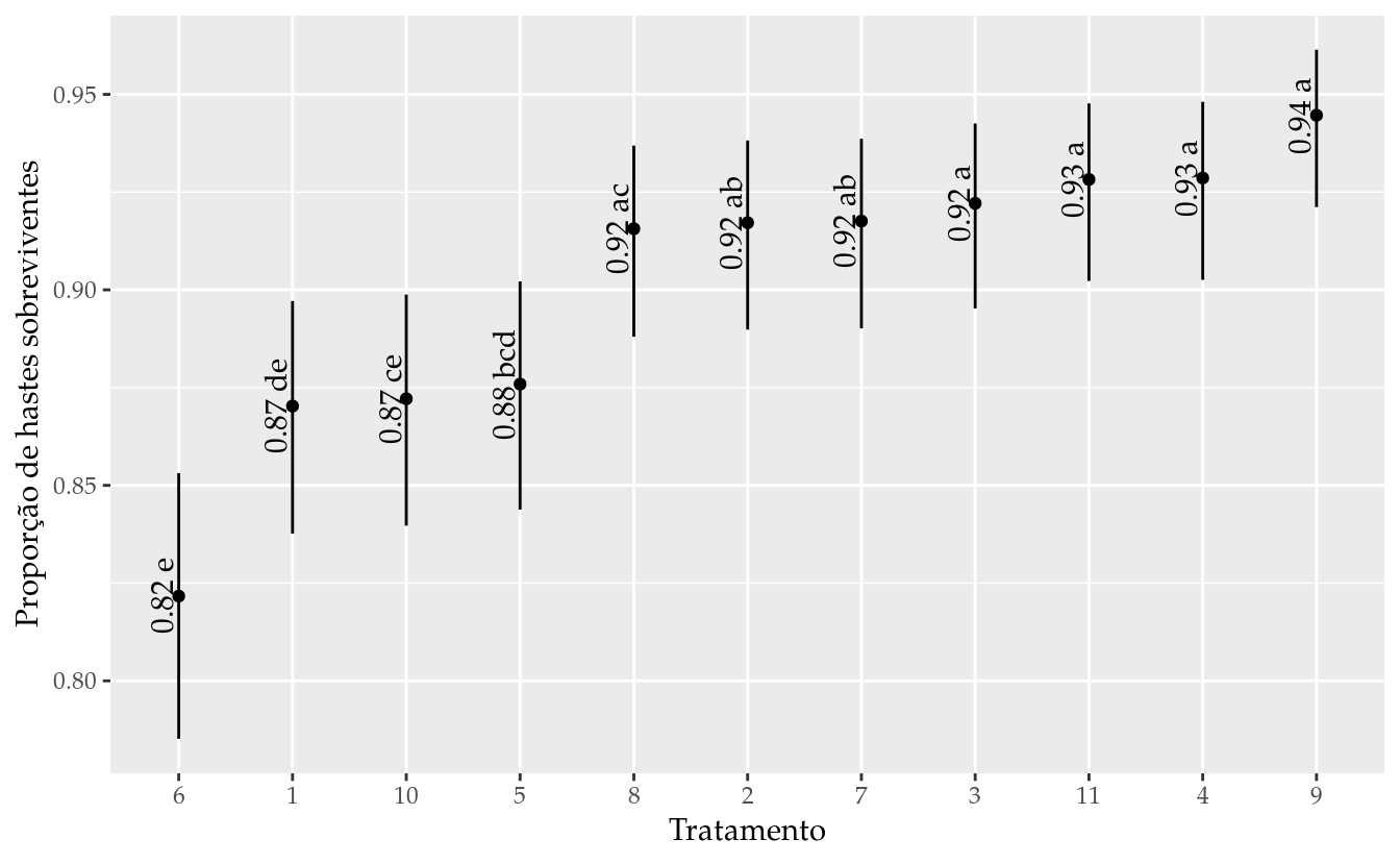
4.5 Geração do delineamento
latin_square(6)## lin col trt
## 1 1 1 6
## 2 2 1 3
## 3 3 1 2
## 4 4 1 4
## 5 5 1 1
## 6 6 1 5
## 7 1 2 2
## 8 2 2 5
## 9 3 2 4
## 10 4 2 6
## 11 5 2 3
## 12 6 2 1
## 13 1 3 1
## 14 2 3 4
## 15 3 3 3
## 16 4 3 5
## 17 5 3 2
## 18 6 3 6
## 19 1 4 3
## 20 2 4 6
## 21 3 4 5
## 22 4 4 1
## 23 5 4 4
## 24 6 4 2
## 25 1 5 5
## 26 2 5 2
## 27 3 5 1
## 28 4 5 3
## 29 5 5 6
## 30 6 5 4
## 31 1 6 4
## 32 2 6 1
## 33 3 6 6
## 34 4 6 2
## 35 5 6 5
## 36 6 6 3TODO!
Manual de Planejamento e Análise de Experimentos com R
Walmes Marques Zeviani